Appendices¶

Internal Input Parameters/Switches¶

The parameter list is handled internally and is populated based on options prescribed in the .par file. In general, it is not recommend for users to override these parameters as their usage may be subject to change. However they can be set or referenced in the .usr file via the param() array. This list was explicitly set with the legacy .rea format.

Parameters¶

P001  density for the case of constant properties

P002  dynamic viscosity

P007  heat capacity for the case of constant properties

P008  conductivity for the case of constant properties

P010  simulation end time

P011  number of time steps

P012  time step size

P014  time fequency to dump fld files

P015  step frequency to dump fld files

P021  pressure solver tolernace

P022  velocity solver tolerance

P023  number of passive scalars

P024  relative tolerance for Helmholtz solver

P025  absolute tolerance for Helmholtz solver

P026  target Courant number (determines the number of RK4 substeps for OIFS)

P027  temporal discretization order

P028  temporal discretization order for mesh solver

P029  magnetic viscosity

P030  material properties (0: constant, 1: uservp)

P031  number of perturbation modes in linearized N-S.

P032  number of boundary conditions in .re2 file

P033  first field index in .re2

P040  pressure coarse grid solver (0: XXT, 1: AMG)

P041 1 \(\rightarrow\) multiplicative SEMG

P042 linear solver for the pressure equation (0: GMRES, 1: CG)

P043 0: additive multilevel scheme - 1: original two level scheme.

P044 0=E-based additive Schwarz for PnPn-2; 1=A-based.

P045 Free-surface stability control (defaults to 1.0)

P046 if \(>0\), do not set Initial Condition (no call to subroutine SETICS).

P047 Poisson ratio for mesh elasticity solve (default 0.4)

P054 direction of fixed flowrate (1: x, 2: y, 3: z), negative means fixed bulk velocity

P055 volumetric flowrate or bulk velocity (see p054) for periodic case

P059 deformed element switch

P060 initialize velocity to 1e-10 (for steady Stokes problem).

P062 byte swap for output

P063 output precision (4: SP, 8: DP)

P064 restart perturbation solution

P065 number of I/O nodes (if \(< 0\) write in separate subdirectories).

P066 output format (0: ASCII, 4: legacy binary, 6: binary)

P067 read format

P068 averaging frequency in avg_all (0: every timestep).

P084 custom inital time step

P086 use skew-symmetric instead of convective form.

P093 number of previous solutions to use for residual projection.

P094 number of steps starting residual projection for velocity and passive scalars

P095 number of steps starting residual projection for pressure

P099 dealiasing mode (\(<0\): disabled, 3: old dealiasing, 4: new dealiasing)

P100 RESERVED! pressure preconditioner when using CG solver (0: Jacobi, \(>0\): two-level Schwarz) or viseversa?

P101 number of additional modes to filter

P103 filter weight for last mode

P107 if \(\neq0\), add it to h2 in sethlm

P116 NELX number of elements in \(x\) for FTP

P117 NELY number of elements in \(y\) for FTP

P118 NELZ number of elements in \(z\) for FTP

Logical switches¶

Like the parameter list, the logical switches are handled internally based on options set in the .par file and it is not recommended for the user to override these settings.

IFFLOW solve for fluid (velocity, pressure)

IFHEAT solve for heat (temperature and/or scalars)

IFTRAN solve transient equations (otherwise, solve the steady Stokes flow)

IFADVC specify the fields with convection

IFTMSH specify the field(s) defined on T mesh (first field is the ALE mesh)

IFAXIS axisymmetric formulation

IFSTRS use stress formulation

IFLOMACH use low Mach number formulation

IFMGRID moving grid

IFMVBD moving boundary (for free surface flow)

IFCHAR use characteristics for convection operator

IFSYNC use upfront synchronization

IFUSERVP user-defined properties

IFXYO include coordinates in output files

IFPO include pressure field in output files

IFVO include velocity fields in output files

IFTO include temperature field in output files

IFPSCO include passive scalar fields in output files, ifpsco(ldimt1)

Commonly Used Variables¶

Solution Variables¶

Table 33 Solution Variables¶
Name	Size	Type	Short Description
`vx`	(lx1,ly1,lz1,lelv)	real	x-velocity (\(u\))
`vy`	(lx1,ly1,lz1,lelv)	real	y-velocity (\(v\))
`vz`	(lx1,ly1,lz1,lelv)	real	z-velocity (\(w\))
`pr`	(lx2,ly2,lz2,lelv)	real	pressure (\(P\))
`t`	(lx1,ly1,lz1,lelt,ldimt)	real	temperature (\(T\)) and passives calars (\(\phi_i\))
`vtrans`	(lx1,ly1,lz1,lelt,ldimt+1)	real	convective coefficient – \(\rho\), \((\rho c_p)\), \(\rho_i\)
`vdiff`	(lx1,ly1,lz1,lelt,ldimt+1)	real	diffusion coefficient – \(\mu\), \(\lambda\), \(\Gamma_i\)
`vxlag`	(lx1,ly1,lz1,lelv,2)	real	\(u\) at previous time steps
`vylag`	(lx1,ly1,lz1,lelv,2)	real	\(v\) at previous time steps
`vzlag`	(lx1,ly1,lz1,lelv,2)	real	\(w\) at previous time steps
`prlag`	(lx2,ly2,lz2,lelv,lorder2)	real	\(P\) at previous time steps
`tlag`	(lx1,ly1,lz1,lelv,lorder-1,ldimt+1)	real	\(T\) and \(\phi_i\) at previous time steps
`time`	–	real	physical time
`dt`	–	real	time step size
`dtlag`		real	previous time step sizes
`istep`	–	integer	time step number

Geometry Variables¶

Variable Name	Size	Type	Short Description
`xm1`	(lx1,ly1,lz1,lelt)	real	x-coordinates for velocity mesh
`ym1`	(lx1,ly1,lz1,lelt)	real	y-coordinates for velocity mesh
`zm1`	(lx1,ly1,lz1,lelt)	real	z-coordinates for velocity mesh
`bm1`	(lx1,ly1,lz1,lelt)	real	mass matrix for velocity mesh
`binvm1`	(lx1,ly1,lz1,lelv)	real	inverse mass matrix for velocity mesh
`bintm1`	(lx1,ly1,lz1,lelt)	real	inverse mass matrix for t mesh
`volvm1`	–	real	total volume for velocity mesh
`voltm1`	–	real	total volume for t mesh
`xm2`	(lx2,ly2,lz2,lelv)	real	x-coordinates for pressure mesh
`ym2`	(lx2,ly2,lz2,lelv)	real	y-coordinates for pressure mesh
`zm2`	(lx2,ly2,lz2,lelv)	real	z-coordinates for pressure mesh
`unx`	(lx1,ly1,6,lelt)	real	x-component of face unit normal
`uny`	(lx1,ly1,6,lelt)	real	y-component of face unit normal
`unz`	(lx1,ly1,6,lelt)	real	z-component of face unit normal
`area`	(lx1,ly1,6,lelt)	real	face area (surface integral weights)

Problem Setup Variables¶

Variable Name	Size	Type	Short Description
`nid`	–	integer	MPI rank id (lowest rank is always 0)
`nio`	–	integer	I/O node id
`nelv`	–	integer	number of elements in velocity mesh
`nelt`	–	integer	number of elements in t mesh
`ndim`	–	integer	dimensionality of problem (i.e. 2 or 3)
`nsteps`	–	integer	number of time steps to run
`iostep`	–	integer	time steps between data output
`cbc`	(6,lelt,ldimt+1)	character*3	boundary condition
`lglel`	(lelt)	integer	local to global element number map
`gllel`	(lelg)	integer	global to local element number map

Averaging Variables¶

Arrays associated with the avg_all subroutine

Variable Name	Size	Type	Short Description
`uavg`	(ax1,ay1,az1,lelt)	real	time averaged x-velocity
`vavg`	(ax1,ay1,az1,lelt)	real	time averaged y-velocity
`wavg`	(ax1,ay1,az1,lelt)	real	time averaged z-velocity
`pavg`	(ax2,ay2,az2,lelt)	real	time averaged pressure
`tavg`	(ax1,ay1,az1,lelt,ldimt)	real	time averaged temperature and passive scalars
`urms`	(ax1,ay1,az1,lelt)	real	time averaged u^2
`vrms`	(ax1,ay1,az1,lelt)	real	time averaged v^2
`wrms`	(ax1,ay1,az1,lelt)	real	time averaged w^2
`prms`	(ax1,ay1,az1,lelt)	real	time averaged pr^2
`trms`	(ax1,ay1,az1,lelt,ldimt)	real	time averaged t^2 and ps^2
`uvms`	(ax1,ay1,az1,lelt)	real	time averaged uv
`vwms`	(ax1,ay1,az1,lelt)	real	time averaged vw
`wums`	(ax1,ay1,az1,lelt)	real	time averaged wu
`iastep`	–	integer	time steps between averaged data output

Commonly used Subroutines¶

subroutine cmult(x,C,n): multiplies n elements of array x by a constant, C.
subroutine rescale_x(x,x0,x1): Rescales the array x to be in the range (x0,x1). This is usually called from usrdat2 in the .usr file.
subroutine normvc(h1,semi,l2,linf,x1,x2,x3): Computes the error norms of a vector field variable (x1,x2,x3) defined on mesh 1, the velocity mesh. The error norms are normalized with respect to the volume, with the exception on the infinity norm, linf.
subroutine comp_vort3(vort,work1,work2,u,v,w): Computes the vorticity (vort) of the velocity field, (u,v,w)
subroutine lambda2(l2): Generates the Lambda-2 vortex criterion proposed by Jeong and Hussain (1995)
subroutine planar_average_z(ua,u,w1,w2): Computes the r-s planar average of the quantity u.
subroutine torque_calc(scale,x0,ifdout,iftout): Computes torque about the point x0. Here scale is a user supplied multiplier so that the results may be scaled to any convenient non-dimensionalization. Both the drag and the torque can be printed to the screen by switching the appropriate ifdout(drag) or iftout(torque) logical.
subroutine set_obj: Defines objects for surface integrals by changing the value of hcode for future calculations. Typically called once within userchk (for istep = 0) and used for calculating torque. (see above)

subroutine avg1(avg,f, alpha,beta,n,name,ifverbose)

subroutine avg2(avg,f, alpha,beta,n,name,ifverbose)

subroutine avg3(avg,f,g, alpha,beta,n,name,ifverbose): These three subroutines calculate the (weighted) average of f. Depending on the value of the logical, ifverbose, the results will be printed to standard output along with name. In avg2, the f component is squared. In avg3, vector g also contributes to the average calculation.
subroutine outpost(x,vy,vz,pr,tz,' '): Dumps the current data of x, vy, vz, pr, tz to an .fld or .f0???? file for post processing.
subroutine platform_timer(ivrb): Runs the battery of timing tests for matrix-matrix products,contention-free processor-to-processor ping-pong tests, and mpi_all_reduce times. Allows one to check the performance of the communication routines used on specific platforms.
subroutine quickmv: Moves the mesh to allow user affine motion.
subroutine runtimeavg(ay,y,j,istep1,ipostep,s5): Computes, stores, and (for ipostep!0) prints runtime averages of j-quantity y (along w/ y itself unless ipostep<0) with j + ‘rtavg_’ + (unique) s5 every ipostep for istep>=istep1. s5 is a string to append to rtavg_ for storage file naming.
subroutine lagrng(uo,y,yvec,uvec,work,n,m): Compute Lagrangian interpolant for uo
subroutine opcopy(a1,a2,a3,b1,b2,b3): Copies b1 to a1, b2 to a2, and b3 to a3, when ndim = 3,
subroutine cadd(a,const,n): Adds const to vector a of size n.
subroutine col2(a,b,n): For n entries, calculates a=a*b.
subroutine col3(a,b,c,n): For n entries, calculates a=b*c.

function glmax(a,n)

function glamax(a,n)

function iglmax(a,n): Calculates the (absolute) max of a vector that is size n. Prefix i implies integer type.
function i8glmax(a,n): Calculates the max of an integer*8 vector that is size n.

function glmin(a,n)

function glamin(a,n)

function iglmin(a,n): Calculates the (absolute) min of a vector that is size n. Prefix i implies integer type.

function glsc2(a,b,n)

function glsc3(a,b,mult,n)

function glsc23(a,b,c,n)

function glsum(a,n)

Computes the global sum of the real arrays a, with number of local entries n

function iglsum(a,n)

Computes the global sum of the integer arrays a, with number of local entries n

function i8glsum(a,n)

Computes the global sum of the integer*8 arrays a, with number of local entries n

subroutine surface_int(dphi,dS,phi,ielem,iside): Computes the surface integral of scalar array phi over face iside of element ielem. The resulting integral is storted in dphi and the area in dS.

Mesh Modification¶

For complex shapes, it is often convenient to modify the mesh direction in the simulation code, Nek5000. This can be done through the usrdat2 routine provided in the .usr file. The routine usrdat2 is called by Nek5000 immediately after the geometry, as specified by the .rea file, is established. Thus, one can use the existing geometry to map to a new geometry of interest.

For example, suppose you want the above pipe geometry to have a sinusoidal wall. Let \({\bf x} := (x,y)\) denote the old geometry, and \({\bf x}' := (x',y')\) denote the new geometry. For a domain with \(y\in [0,0.5]\), the following function will map the straight pipe geometry to a wavy wall with amplitude \(A\), wavelength \(\lambda\):

\[y'(x,y) = y + y A \sin( 2 \pi x / \lambda ).\]

Note that, as \(y \longrightarrow 0\), the perturbation, \(yA \sin( 2 \pi x / \lambda )\), goes to zero. So, near the axis, the mesh recovers its original form.

In Nek5000, you would specify this through usrdat2 as follows

subroutine usrdat2
include 'SIZE'
include 'TOTAL'

real lambda

ntot = nx1*ny1*nz1*nelt

lambda = 3.
A      = 0.1

do i=1,ntot
   argx         = 2*pi*xm1(i,1,1,1)/lambda
   ym1(i,1,1,1) = ym1(i,1,1,1) + ym1(i,1,1,1)*A*sin(argx)
end do

param(59) = 1.  ! Force nek5 to recognize element deformation.

return
end

Note that, since Nek5000 is modifying the mesh, postx will not recognize the current mesh unless you tell it to, because postx looks to the .rea file for the mesh geometry. The only way for Nek5000 to communicate the new mesh to postx is via the .fld file, so you must request that the geometry be dumped to the .fld file. The result of above changes is shown in Fig. 32.

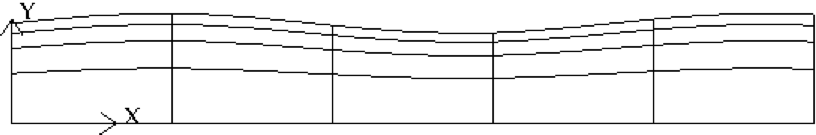
Fig. 32 Axisymmetric pipe mesh.

Cylindrical/Cartesian-transition Annuli¶

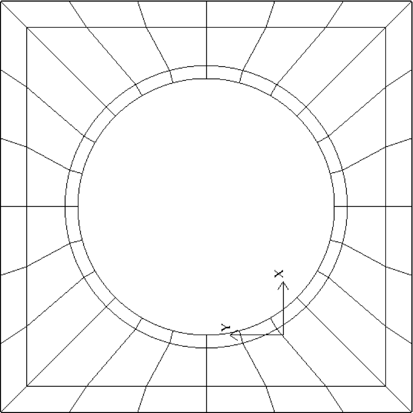
Fig. 33 Cylinder mesh

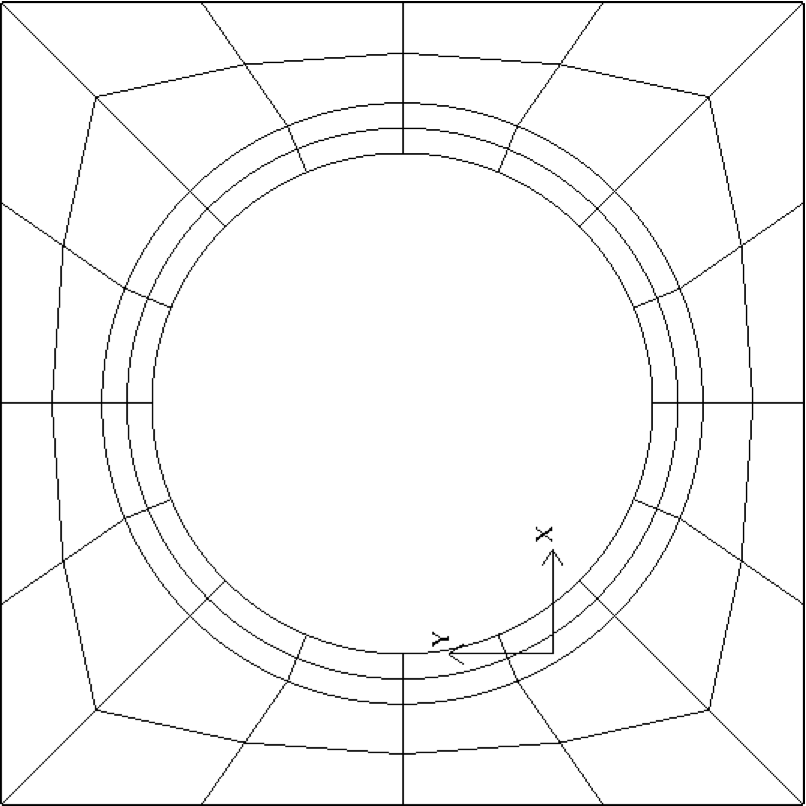
Fig. 34 Cylinder mesh

More sophisticated transition treatments may be generated using the GLOBAL REFINE options in preNek or through an upgrade of genb7, as demand warrants. Example 2D and 3D input files are provided in the nek5000/doc files box7.2d and box7.3d. Fig. 33 shows a 2D example generated using the box7.2d input file, which reads:

x2d.rea
2                      spatial dimension
1                      number of fields
#
#    comments
#
#
#========================================================
#
Y                   cYlinder
3 -24 1             nelr,nel_theta,nelz
.5 .3               x0,y0 - center of cylinder
ccbb                descriptors: c-cyl, o-oct, b-box (1 character + space)
.5 .55 .7 .8        r0 r1 ... r_nelr
0  1  1             theta0/2pi theta1/2pi  ratio
v  ,W  ,E  ,E  ,    bc's (3 characters + comma)

An example of a mesh is shown in Fig. 33. The mesh has been quad-refined once with oct-refine option of preNek. The 3D counterpart to this mesh could joined to a hemisphere/Cartesian transition built with the spherical mesh option in preNek.