Theory

Computational Approach

The spatial discretization is based on the spectral element method (SEM) [Patera1984], which is a high-order weighted residual technique similar to the finite element method. In the SEM, the solution and data are represented in terms of \(N^{th}\)-order tensor-product polynomials within each of \(E\) deformable hexahedral (brick) elements. Typical discretizations involve \(E=\) 100–1,000,000 elements of order \(N=\) 8–16 (corresponding to 512–4096 points per element). Vectorization and cache efficiency derive from the local lexicographical ordering within each macro-element and from the fact that the action of discrete operators, which nominally have \(O(EN^6)\) nonzeros, can be evaluated in only \(O(EN^4)\) work and \(O(EN^3)\) storage through the use of tensor-product-sum factorization [Orszag1980]. The SEM exhibits very little numerical dispersion and dissipation, which can be important, for example, in stability calculations, for long time integrations, and for high Reynolds number flows. We refer to [Denville2002] for more details.

Nek5000 solves the unsteady incompressible two-dimensional, axisymmetric, or three-dimensional Stokes or Navier-Stokes equations with forced or natural convection heat transfer in both stationary (fixed) or time-dependent geometry. It also solves the compressible Navier-Stokes in the Low Mach regime, and the magnetohydrodynamic equation (MHD). The solution variables are the fluid velocity \(\mathbf u=(u_{x},u_{y},u_{z})\), the pressure \(p\), the temperature \(T\). All of the above field variables are functions of space \({\bf x}=(x,y,z)\) and time \(t\) in domains \(\Omega_f\) and/or \(\Omega_s\) defined in Fig. 31. Additionally Nek5000 can handle conjugate heat transfer problems.

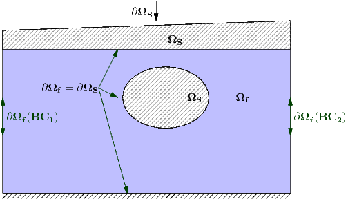
Fig. 31 Computational domain showing respective fluid and solid subdomains, \(\Omega_f\) and \(\Omega_s\). The shared boundaries are denoted \(\partial\Omega_f=\partial\Omega_s\) and the solid boundary which is not shared by fluid is \(\overline{\partial\Omega_s}\), while the fluid boundary not shared by solid \(\overline{\partial\Omega_f}\).

Incompressible Navier-Stokes Equations

The governing equations of flow motion in dimensional form are

(3)\[\rho\left(\frac{\partial\mathbf u}{\partial t} +\mathbf u \cdot \nabla \mathbf u\right) = - \nabla p + \nabla \cdot \boldsymbol{\underline\tau} + \rho {\bf f} \,\, , \text{in } \Omega_f , \quad \text{ (Momentum) }\]

where \(\boldsymbol{\underline\tau}=\mu[\nabla \mathbf u+\nabla \mathbf u^{T}]\) and \(\mathbf f\) is a user defined acceleration.

(4)\[\nabla \cdot \mathbf u =0 \,\, , \text{in } \Omega_f, \quad \text{ (Continuity) }\]

If the fluid viscosity is constant in the entire domain the viscous stress tensor can be contracted using the Laplace operator. Therefore one may solve the Navier–Stokes equations in either the full-stress formulation

(5)\[\nabla \cdot \boldsymbol{\underline\tau}=\nabla \cdot \mu[\nabla \mathbf u+\nabla \mathbf u^{T}]\]

or the no-stress formulation

(6)\[\nabla \cdot \boldsymbol{\underline\tau}=\mu\Delta \mathbf u\]

• Variable viscosity and RANS models require the full-stress tensor.
• Constant viscosity leads to a simpler stress tensor, which we refer to as the ‘no-stress’ formulation.

Non-Dimensional Navier-Stokes

Let us introduce the following non-dimensional variables \(\mathbf x^*\ = \frac{\mathbf x}{L_0}\), \(\mathbf u^*\ = \frac{u}{u_0}\), \(t^*\ = \frac{tu_0}{L_0}\), and \(\mathbf f^* =\frac{\mathbf f L_0}{u_0^2}\). Where \(L_0\) and \(u_0\) are the (constant) characteristic length and velocity scales, respectively. For the pressure scale we have two options:

• Convective effects are dominant i.e. high velocity flows \(p^* = \frac{p}{\rho u_0^2}\)
• Viscous effects are dominant i.e. creeping flows (Stokes flow) \(p^* = \frac{p L_0}{\mu_0 u_0}\),

where \(\mu_0\) is a constant reference value for molecular viscosity. For highly convective flows we choose the first scaling of the pressure and obtain the non-dimensional Navier-Stokes in the no-stress formulation:

(7)\[\frac{\partial \mathbf{u^*}}{\partial t^*} + \mathbf{u^*} \cdot \nabla \mathbf{u^*}\ = -\nabla p^* + \frac{1}{Re}\Delta\mathbf u^* + \mathbf f^*.\]

For the full-stress formulation, we further introduce the dimensionless viscosity, \(\mu^*=\frac{\mu}{\mu_0}\), and obtain:

(8)\[\frac{\partial \mathbf{u^*}}{\partial t^*} + \mathbf{u^*} \cdot \nabla \mathbf{u^*}\ = -\nabla p^* + \frac{1}{Re}\nabla \cdot \left[ \mu^* \left(\nabla\mathbf u^* + \nabla\mathbf u^{* T}\right)\right] + \mathbf f^*,\]

where \(\mathbf f^*\) is the dimensionless user defined forcing function. The non-dimensional number here is the Reynolds number \(Re=\frac{\rho u_0 L_0}{\mu_0}\).

Energy Equation

In addition to the fluid flow, Nek5000 computes automatically the energy equation

(9)\[\rho c_{p} \left( \frac{\partial T}{\partial t} + \mathbf u \cdot \nabla T \right) = \nabla \cdot (\lambda \nabla T) + q''', \quad \text{in } \Omega_f\cup \Omega_s \text{ (Energy) }\]

Non-Dimensional Energy / Passive Scalar Equation

A similar non-dimensionalization as for the flow equations using the non-dimensional variables \(\mathbf x^*\ = \frac{\mathbf x}{L_0}\), \(\mathbf u^*\ = \frac{u}{u_0}\), \(t^*\ = \frac{tu_0}{L_0}\), \(T=\frac{T^*-T_0}{\delta T_0}\), and \(\lambda^*=\frac{\lambda}{\lambda_0}\) leads to

(10)\[\frac{\partial T^*}{\partial t^*} + \mathbf u^* \cdot \nabla T^* = \frac{1}{Pe} \nabla \cdot \lambda^*\nabla T^* + q^*, \quad \text{in } \Omega_f\cup \Omega_s \text{ (Energy) }\]

where \(q^*=\frac{q''' L_0}{\rho c_p u_0 \delta T_0}\) is the dimensionless user defined source term. The non-dimensional number here is the Peclet number, \(Pe=\frac{\rho c_p u_0 L_0}{\lambda_0}\).

Passive Scalars

We can additionally solve a convection-diffusion equation for each passive scalar \(\phi_i\), \(i = 1,2,\ldots\) in \(\Omega_f \cup \Omega_s\)

(11)\[\rho_i \left( \frac{\partial \phi_{i}}{\partial t} + \mathbf u \cdot \nabla \phi_{i} \right) = \nabla \cdot (\Gamma_i \nabla \phi_{i}) + (q''')_i.\]

The terminology and restrictions of the temperature equations are retained for the passive scalars, so that it is the responsibility of the user to convert the notation of the passive scalar parameters to their thermal analogues. For example, in the context of mass transfer, the user should recognize that the values specified for temperature and heat flux will represent concentration and mass flux, respectively. Any combination of these equation characteristics is permissible with the following restrictions. First, the equation must be set to unsteady if it is time-dependent or if there is any type of advection. For these cases, the steady-state (if it exists) is found as stable evolution of the initial-value-problem. Secondly, the stress formulation must be selected if the geometry is time-dependent. In addition, stress formulation must be employed if there are traction boundary conditions applied on any fluid boundary, or if any mixed velocity/traction boundaries, such as symmetry and outflow/n, are not aligned with either one of the Cartesian \(x,y\) or \(z\) axes. Other capabilities of Nek5000 are the linearized Navier-Stokes for flow stability, magnetohydrodynamic flows etc.

Unsteady Stokes

In the case of flows dominated by viscous effects Nek5000 can solve the reduced Stokes equations

(12)\[\rho\left(\frac{\partial \mathbf u}{\partial t} \right) = - \nabla p + \nabla \cdot \boldsymbol{\underline\tau} + \rho {\bf f} \,\, , \text{in } \Omega_f \text{ (Momentum) }\]

where \(\boldsymbol{\underline\tau}=\mu[\nabla \mathbf u+\nabla \mathbf u^{T}]\) and

(13)\[\nabla \cdot \mathbf u =0 \,\, , \text{in } \Omega_f \text{ (Continuity) }\]

Also here we can distinguish between the stress and non-stress formulation according to whether the viscosity is variable or not. The non-dimensional form of these equations can be obtained using the viscous scaling of the pressure.

Steady Stokes

If there is no time-dependence, then Nek5000 can further reduce to

(14)\[- \nabla p + \nabla \cdot \boldsymbol{\underline\tau} + \rho {\bf f}=0 \,\, , \text{in } \Omega_f \text{ (Momentum) }\]

where \(\boldsymbol{\underline\tau}=\mu[\nabla \mathbf u+\nabla {\mathbf u}^{T}]\) and

(15)\[\nabla \cdot \mathbf u =0 \,\, , \text{in } \Omega_f \text{ (Continuity) }\]

Linearized Equations

In addition to the basic evolution equations described above, Nek5000 provides support for the evolution of small perturbations about a base state by solving the linearized equations

(16)\[\begin{split}\rho\left(\frac{\partial \mathbf u_i'}{\partial t} + \mathbf u \cdot \nabla {\mathbf u_i}^{'} + \mathbf u_i' \cdot \nabla \mathbf u \right) &= - \nabla p_i' + \mu \nabla^2 \mathbf u_i'\\ \nabla \cdot \mathbf u_i' &= 0 \nonumber\end{split}\]

for multiple perturbation fields \(i=1,2,\dots\) subject to different initial conditions and (typically) homogeneous boundary conditions.

These solutions can be evolved concurrently with the base fields \((\mathbf u,p,T)\). There is also support for computing perturbation solutions to the Boussinesq equations for natural convection. Calculations such as these can be used to estimate Lyapunov exponents of chaotic flows, etc.

Steady Conduction

The energy equation (9) in which the advection term \(\mathbf u \cdot \nabla T\) and the transient term \(\partial T/\partial t\) are zero. In essence this represents a Poisson equation.

Low-Mach Navier-Stokes

The compressible Navier-Stokes differ mathematically from the incompressible ones mainly in the divergence constraint \(\nabla \cdot \mathbf u\neq 0\). In this case the system of equations is not closed and an additional equation of state (EOS) is required to connect the state variables, e.g. \(\rho=f(p,T)\). Nek5000 includes the ability to solve the low-Mach approximation of the compressible Navier-Stokes, \(\rho\approx f(T)\). The low-Mach approximation decouples the pressure from the velocity leading to a system of equations which can be solved numerically in a similar fashion as the incompressible Navier-Stokes.

The low-Mach equations are

(17)\[\begin{split}\rho\left(\frac{\partial \mathbf u}{\partial t}+ \mathbf u\cdot\nabla\mathbf u\right)&=-\nabla p+\nabla \cdot\boldsymbol{\underline\tau}+\rho\mathbf f\ \\ \nabla \cdot \mathbf u &= -\frac{1}{\rho}\frac{\mathrm d \rho}{\mathrm d T}\left(\frac{\partial T}{\partial t}+ \mathbf u\cdot\nabla T\right) \\ \rho c_p\left(\frac{\partial T}{\partial t}+ \mathbf u\cdot\nabla T\right)&=-\nabla \cdot k \nabla T + q'''\end{split}\]

where \(\boldsymbol{\underline\tau}=\mu[\nabla \mathbf u+\nabla \mathbf u^{T}-\frac{2}{3}\nabla \cdot \mathbf u \mathbf I]\).

This allows for both variable density and variable viscosity. The system is solved by substituting \(\rho\approx f(T)\) into the continuity equation and obtaining a so-called thermal divergence.

Incompressible MHD Equations

Magnetohydrodynamics is based on the idea that magnetic fields can induce currents in a moving conductive fluid, which in turn creates forces on the fluid and changing the magnetic field itself. The set of equations which describe MHD are a combination of the Navier-Stokes equations of fluid dynamics and Maxwell’s equations of electromagnetism. These differential equations have to be solved simultaneously, and Nek5000 has an implementation for the incompressible MHD.

Consider a fluid of velocity \(\mathbf u\) subject to a magnetic field \(\mathbf B\) then the incompressible MHD equations are

(18)\[\begin{split}\rho\left(\frac{\partial\mathbf u}{\partial t} + \mathbf u \cdot \nabla \mathbf u\right) &= - \nabla p + \mu \Delta \mathbf u + \mathbf B\cdot \nabla \mathbf B \ ,\\ \nabla \cdot \mathbf u &= 0\\ \nonumber \frac{\partial \mathbf B}{\partial t} + \mathbf u \cdot \nabla \mathbf B &= - \nabla q + \eta \Delta \mathbf B + \mathbf B\cdot \nabla \mathbf u \ ,\\ \nabla \cdot \mathbf B &= 0\end{split}\]

where \(\rho\) is the density \(\mu\) the viscosity, \(\eta\) resistivity, and pressure \(p\).

The total magnetic field can be split into two parts: \(\mathbf{B} = \mathbf{B_0} + \mathbf{b}\) (mean + fluctuations). The above equations become in terms of Elsässer variables (\(\mathbf{z}^{\pm} = \mathbf{u} \pm \mathbf{b}\))

\[\frac{\partial {\mathbf{z}^{\pm}}}{\partial t}\mp\left(\mathbf {B}_0\cdot{\mathbf \nabla}\right){\mathbf z^{\pm}} + \left({\mathbf z^{\mp}}\cdot{\mathbf \nabla}\right){\mathbf z^{\pm}} = -{\mathbf \nabla}p + \nu_+ \nabla^2 \mathbf{z}^{\pm} + \nu_- \nabla^2 \mathbf{z}^{\mp}\]

where \(\nu_\pm = \nu \pm \eta\).

The important non-dimensional parameters for MHD are \(Re = U L /\nu\) and the magnetic Re \(Re_M = U L /\eta\).

Arbitrary Lagrangian-Eulerian (ALE)

We consider unsteady incompressible flow in a domain with moving boundaries:

(19)\[\begin{split}\frac{\partial\mathbf u}{\partial t} = -\nabla p +\frac{1}{Re}\nabla\cdot(\nabla + \nabla^T)\mathbf u + NL,\\ \nabla \cdot \mathbf u = 0\end{split}\]

Here, \(NL\) represents the quadratic nonlinearities from the convective term.

Our free-surface hydrodynamic formulation is based upon the arbitrary Lagrangian-Eulerian (ALE) formulation described in [Ho1989]. Here, the domain \(\Omega(t)\) is also an unknown. As with the velocity, the geometry \(\mathbf x\) is represented by high-order polynomials. For viscous free-surface flows, the rapid convergence of the high-order surface approximation to the physically smooth solution minimizes surface-tension-induced stresses arising from non-physical cusps at the element interfaces, where only \(C^0\) continuity is enforced. The geometric deformation is specified by a mesh velocity \(\mathbf w := \dot{\mathbf x}\) that is essentially arbitrary, provided that \(\mathbf w\) satisfies the kinematic condition \(\mathbf w \cdot \hat{\mathbf n}|^{}_{\Gamma} = \mathbf u \cdot \hat{\mathbf n}|^{}_{\Gamma}\), where \(\hat{\mathbf n}\) is the unit normal at the free surface \(\Gamma(x,y,t)\). The ALE formulation provides a very accurate description of the free surface and is appropriate in situations where wave-breaking does not occur.

To highlight the key aspects of the ALE formulation, we introduce the weighted residual formulation of Eq. (19): Find \((\mathbf u,p) \in X^N \times Y^N\) such that:

(20)\[\frac{\mathrm d}{\mathrm d t}(\mathbf v,\mathbf u) = (\nabla \cdot \mathbf v,p) - \frac{2}{Re}(\nabla \mathbf v,\mathbf S) +(\mathbf v,N\!L) + c(\mathbf v,\mathbf w,\mathbf u), \qquad (\nabla \cdot \mathbf u,q) = 0,\]

for all test functions \((\mathbf v,q) \in X^N \times Y^N\). Here \((X^N,Y^N)\) are the compatible velocity-pressure approximation spaces introduced in [Maday1989], \((.,.)\) denotes the inner-product \((\mathbf f,\mathbf g) := \int_{\Omega(t)} \mathbf f \cdot \mathbf g \,dV\), and \(\mathbf S\) is the stress tensor \(S_{ij}^{} := \frac{1}{2}( \frac{\partial u_i}{\partial x_j} + \frac{\partial u_j}{\partial x_i} )\). For simplicity, we have neglected the surface tension term. A new term in Eq. (20) is the trilinear form involving the mesh velocity

(21)\[c(\mathbf v,\mathbf w,\mathbf u) := \int_{\Omega(t)}^{} \sum_{i=1}^3 \sum_{j=1}^3 v_i^{} \frac{\partial w_j^{} u_i^{}}{\partial x_j^{}} \,dV,\]

which derives from the Reynolds transport theorem when the time derivative is moved outside the bilinear form \((\mathbf v,\mathbf u_t^{})\). The advantage of Eq. (20) is that it greatly simplifies the time differencing and avoids grid-to-grid interpolation as the domain evolves in time. With the time derivative outside of the integral, each bilinear or trilinear form involves functions at a specific time, \(t^{n-q}\), integrated over \(\Omega(t^{n-q})\). For example, with a second-order backward-difference/extrapolation scheme, the discrete form of Eq. (20) is

(22)\[\frac{1}{2 \Delta t}\left[ 3 (\mathbf v^n,\mathbf u^n)^n -4 (\mathbf v^{n-1},\mathbf u^{n-1})^{n-1} + (\mathbf v^{n-2},\mathbf u^{n-2})^{n-2} \right] = L^n (\mathbf u) + 2 \widetilde{N\!L}^{n-1} - \widetilde{N\!L}^{n-2}.\]

Here, \(L^n(\mathbf u)\) accounts for all linear terms in Eq. (20), including the pressure and divergence-free constraint, which are evaluated implicitly (i.e., at time level \(t^n\), on \(\Omega(t^n)\)), and \(\widetilde{N\!L}^{n-q}\) accounts for all nonlinear terms, including the mesh motion term (21), at time-level \(t^{n-q}\). The superscript on the inner-products \((.,.)^{n-q}\) indicates integration over \(\Omega(t^{n-q})\). The overall time advancement is as follows. The mesh position \(\mathbf x^n \in \Omega(t^n)\) is computed explicitly using \(\mathbf w^{n-1}\) and \(\mathbf w^{n-2}\); the new mass, stiffness, and gradient operators involving integrals and derivatives on \(\Omega(t^n)\) are computed; the extrapolated right-hand-side terms are evaluated; and the implicit linear system is solved for \(\mathbf u^n\). Note that it is only the operators that are updated, not the matrices. Matrices are never formed in Nek5000 and because of this, the overhead for the moving domain formulation is very low.

Reynolds Averaged Navier-Stokes Models (Experimental)

Two-equation Reynolds Averaged Navier Stokes (RANS) models rely on the Bousinessq approximation which relates the Reynolds stress tensor to the mean strain rate, \(\boldsymbol{\underline {S}}\), linearly through eddy viscosity. The time-averaged momentum equation is given as,

(23)\[\begin{split}\rho \left(\frac{\partial \mathbf u}{\partial t} + \mathbf u \cdot \nabla \mathbf u \right) &= - \nabla p + \nabla \cdot \left[ (\mu + \mu_t) \left( 2 \boldsymbol{\underline S} - \frac{2}{3} Q \boldsymbol{\underline I}\right) \right] \\ \boldsymbol{\underline S} &= \frac{1}{2} \left( \nabla \mathbf u + \nabla\mathbf{u}^T \right) \nonumber\end{split}\]

where \(\mu_t\) is the turbulent or eddy viscosity and \(\boldsymbol{\underline I}\) is an identity tensor. It only supports incompressible flow where the divergence constraint, \(Q\), is zero,

(24)\[Q = \nabla \cdot \mathbf u = 0\]

In two-equation models, the description of the local eddy viscosity is given by two additional transported variables, which provide the velocity and length (or time) scale of turbulence. The velocity scale is given by turbulent kinetic energy while the choice of the second variable, which provides the length scale, depends on the specific two-equation model used. Nek5000 offers several two-equation RANS models based on the \(k-\omega\) [Wilcox2008] family of models. These include the regularized \(k-\omega\) [Tombo2018] and the \(k-\tau\) [Speziale1992] model. In addition, the SST (shear stress transport) and low-Re variants of both models are available.

Note

All currently available RANS models are wall-resolved models.

The \(k-\tau\) model offers certain favorable characteristics over the \(k-\omega\) model, including bounded asymptotic behavior of \(\tau\) and its source terms and favorable near-wall gradients. These make it especially suited for high-order codes and complex geometries. It is, therefore, the preferred two-equation RANS model in Nek5000. The \(k-\tau\) transport equations are,

(25)\[\begin{split}\rho\left( \frac{\partial k}{\partial t} + \mathbf u \cdot \nabla k\right) & = \nabla \cdot (\Gamma_k \nabla k) + P_k - \rho \beta^* \frac{k}{\tau} \\ \rho\left( \frac{\partial \tau}{\partial t} + \mathbf u \cdot \nabla\tau\right) & = \nabla \cdot (\Gamma_\omega \nabla \tau) - \alpha \frac{\tau}{k}P_k + \rho \beta - 2\frac{\Gamma_\omega}{\tau} (\nabla \tau \cdot \nabla \tau) + C_{D_\tau}\end{split}\]

These are implemented using the passive scalar solver. The diffusion terms are given by

\[\begin{split}\Gamma_k & = \mu + \frac{\mu_t}{\sigma_k} \\ \Gamma_\omega & = \mu + \frac{\mu_t}{\sigma_\omega}\end{split}\]

Where, in the \(k-\tau\) model

\[\mu_t = \rho\alpha^* k \tau\]

The production term is given by

\[P_k = \mu_t\left( \boldsymbol{\underline S : \underline S} \right)\]

where “\(\boldsymbol :\)” denotes the double dot product. The final term in the \(\tau\) equation is the cross-diffusion term, introduced by [Kok2000],

(26)\[C_{D_\tau} =(\rho \sigma_d \tau) \text{min}(\nabla k \cdot \nabla \tau,0)\]

The above term is especially relevant for external flows. It eliminates non-physical free-stream dependence of the near-wall \(\tau\) field.

All coefficients in the \(k-\tau\) model are identical to the \(k-\omega\) model and can be found in [Wilcox2008].

The current RANS implementation is offered on an experimental, as-is basis. It cannot be guaranteed to work with all other features of Nek5000 and is still being tested for robustness. As such, it is not automatically compiled with the base code and the required subroutines will need to be included in the .usr file from the Nek5000/core/experimental directory.