Case Files¶

Each simulation is defined by six required case files:

SESSION.NAME
par (runtime parameters)
re2 (mesh and boundaries)
usr (user defined functions for inital/boundary condition etc.)
SIZE (parameters for static memory allocation)
map/ma2 (element processes mapping)

Additional optional case files may be generated or included:

f%05d (solution data)
his (probing point data)

SESSION.NAME¶

To run Nek5000, each simulation must have a SESSION.NAME file. This file is read in by the code and gives the path to the relevant files describing the structure and parameters of the simulation. It contains the name of the simulation and the full path to supporting files. For example, to run the eddy example from the repository, the SESSION.NAME file would look like:

eddy_uv
/home/user_name/Nek5000/short_tests/eddy/

This file is generated automatically by the nek, nekb, nekmpi, nekbmpi, neknek and neknekb scripts at runtime. If you are calling $ mpirun directly, such as in a submission script for an HPC system, you must manually generate this file or setup your script to generate it for you.

Warning

When using NekNek, SESSION.NAME is substantially different. We recommend running the example and checking the neknek script for further information.

Parameter File (.par)¶

The simulation paramaters are defined in the .par file. The keys are grouped in different sections and a specific value is assigned to each key. The .par file follows the structure exemplified below.

#
# nek parameter file
#

[SECTION]
key = value
...

[SECTION]
key = value
...

The sections are:

GENERAL (mandatory)
PROBLEMTYPE
MESH
VELOCITY
PRESSURE (required for velocity)
TEMPERATURE
SCALAR%%
CVODE

When scalars are used, the keys of each scalar are defined under the section SCALAR%% varying between SCALAR01 and SCALAR99. The descripton of the keys of each section is given in the following tables (all keys/values are case insensitive). The value assigned to each key can be a user input (e.g. a <real> value) or one of the avaliable options listed in the tables below. Values in parentheses denote the default value.

Table 5 `GENERAL` keys in the `.par` file¶
Key	Value(s)	Description
`startFrom`	`<string>`	Absolute/relative path of the field file to restart the simulation from. Also includes several restart options (see Restart Options for details)
`stopAt`	`(numSteps)` `endTime`	Stops the simulation after a given number of time steps or at a given physical time.
`endTime`	`<real>`	Final physical time at which we want to our simulation to stop. Required for `stopAt = endTime`.
`numSteps`	`<int>`	Number of time steps until the simulation stops. Required for `stopAt = numSteps`.
`dt`	`<real>`	Specifies the step size or in case of a variable time step, the maximum step size
`variableDT`	`(no)` `yes`	Controls if the step size will be adjusted to match the targetCFL.
`initialDT`	`<real>`	Controls the initial time step size. Requires `variableDT = yes`.
`targetCFL`	`<real>`	Sets stability/target CFL number for OIFS or variable time steps. This is fixed to 0.5 for `extrapolation = standard`
`writeControl`	`(timeStep)` `runTime`	Specifies whether checkpointing is based on number of time steps or physical time.
`writeInterval`	`<real>/<int>`	Checkpoint frequency in physical time (`<real>`) or number of time steps (`<int>`)
`filtering`	`(none)` `explicit` `hpfrt`	Specifies the filtering method. See Stabilizing Filters for details.
`filterModes`	`<int>`	Specifies the number of modes filtered as an alternative to specifying the cutoff ratio. Note: requires the use of at least 2 modes. See Stabilizing Filters for details.
`filterCutoffRatio`	`<real>`	Ratio of modes not affected by the filter. Use as an alternative to specifying the number of modes explicitly. See Stabilizing Filters for details.
`filterWeight`	`<real>`	Sets the filter strength of transfer function of the last mode (explicit) or the relaxation parameter in case of hpfrt. See Stabilizing Filters for more information.
`writeDoublePrecision`	`no` `(yes)`	Sets the precision of the output field files.
`writeNFiles`	`<int>` `(1)`	Sets the number of output files. By default a parallel shared file is used.
`dealiasing`	`no` `yes`	Enable/diasble over-integration.
`timeStepper`	`BDF1` `(BDF2)` `BDF3`	Time integration order.
`extrapolation`	`(standard)` `OIFS`	Extrapolation method. Can be used to achieve CFL > 0.5 with `OIFS`.
`constFlowRate`	`(none)` `X` `Y` `Z`	Prescribes a constant volumetric flow in the given direction. Requires `meanVolumetricFlow` or `meanVelocity`.
`meanVolumetricFlow`	`<real>`	Sets the volumetric flow rate in the direction of `constFlowRate`.
`meanVelocity`	`<real>`	Sets the mean velocity (volume-weighted velocity mean) in the direction of `constFlowRate`.
`optLevel`	`<int>` `(2)`	Optimization level
`logLevel`	`<int>` `(2)`	Controls the verbosity level of the logfile.
`userParam%%`	`<real>`	User parameter (can be accessed through uparam(%) array in `.usr`. Supports up to 20 parameters.

Table 6 `PROBLEMTYPE` keys in the `.par` file¶
Key	Value(s)	Description
`equation`	`(incompNS)` `lowMachNS` `steadyStokes` `incompLinNS` `incompLinAdjNS` `incompMHD` `compNS`	Specifies equation type
`axiSymmetry`	`(no)` `yes`	Axisymmetric problem
`swirl`	`(no)` `yes`	Enable axisymmetric azimuthal velocity component (stored in temperature field
`cyclicBoundaries`	`(no)` `yes`	Sets cyclic periodic boundaries
`numberOfPerturbations`	`(1)`	Number of perturbations for linearized NS
`solveBaseFlow`	`(no)` `yes`	Solve for base flow in case of linearized NS
`variableProperties`	`(no)` `yes`	Enable variable transport properties
`stressFormulation`	`(no)` `yes`	Enable stress formulation
`dp0dt`	`(no)` `yes`	Enable time-varying thermodynamic pressure

Table 7 `COMMON` keys for all field variables in the `.par` file¶
Key	Value(s)	Description
`residualTol`	`<real>`	Residual tolerance used by solver (not for CVODE)
`residualProj`	`(no)` `yes`	Controls the residual projection
`writeToFieldFile`	`no` `(yes)`	Controls if fields will be written on output

Table 8 `MESH` keys in the `.par` file¶
Key	Value(s)	Description
`motion`	`(none)` `user` `elasticity`	Mesh motion solver
`viscosity`	`(0.4)`	Diffusivity for elasticity solver
`numberOfBCFields`	`(nfields)`	Number of field variables which have a boundary condition in `.re2` file
`firstBCFieldIndex`	`(1 or 2)`	Field index of the first BC specified in `.re2` file

Table 9 `VELOCITY` keys in the `.par` file¶
Key	Value(s)	Description
`viscosity`	`<real>`	Dynamic viscosity A negative value sets the Reynolds number
`density`	`<real>`	Density

Table 10 `PRESSURE` keys in the `.par` file¶
Key	Value(s)	Description
`preconditioner`	`(semg_xxt)`	Standard preconditioning method. Requires no additional setup. Only recommended for problems with $E<350,000$.
–	`semg_amg`	First time usage of `semg_amg` with write three dump files to disc. The `amg_hypre` tool will then need to be run to create the setup files required for the AMG solver initialization.
–	`semg_amg_hypre`	Recommended for $E≥350,000$. Requires compiling with HYPRE support.
–	`fem_amg_hypre`	May be faster for meshes with high aspect ratios. Requires compiling with HYPRE support.
`solver`	`(GMRES)` `CGFLEX`	Solver for pressure

Table 11 `COMMON` keys for temperature and scalar fields in the `.par` file¶
Key	Value(s)	Description
`solver`	`(helm)` `cvode` `none`	Solver for scalar
`advection`	`no` `(yes)`	Controls if advection is present
`absoluteTol`	`<real>`	Absolute tolerance used by CVODE

Table 12 `TEMPERATURE` keys in the `.par` file¶
Key	Value(s)	Description
`ConjugateHeatTransfer`	`(no)` `yes`	Controls conjugate heat transfer
`conductivity`	`<real>`	Thermal conductivity
`rhoCp`	`<real>`	Product of density and heat capacity

Note: [TEMPERATURE] solver = none is incompatible with [PROBLEMTYPE] equation = lowMachNS without defining a custom thermal divergence in the usr file.

Table 13 `SCALAR%%` keys in the `.par` file¶
Key	Value(s)	Description
`density`	`<real>`	Density
`diffusivity`	`<real>`	Diffusivity

Table 14 `CVODE` keys in the `.par` file¶
Key	Value(s)	Description
`relativeTol`	`<real>`	Relative tolerance (applies to all scalars)
`stiff`	`no` `(yes)`	Controls if BDF or Adams Moulton is used
`preconditioner`	`(none)` `user`	Preconditioner method
`dtMax`	`<real>`	Maximum internal step size Controls splitting error of velocity scalar coupling (e.g. set to 1-4 dt)

Mesh File (.re2)¶

Stores the mesh and boundary condition.

TODO: Update to re2

Element data¶

Table 15 Geometry description in .rea file¶

ELEMENT 1 [ 1A] GROUP 0

Face {1,2,3,4}

$x_{1,\ldots,4}=$ 0.000000E+00 0.171820E+00 0.146403E+00 0.000000E+00

$y_{1,\ldots,4}=$ 0.190000E+00 0.168202E+00 0.343640E+00 0.380000E+00

$z_{1,\ldots,4}=$ 0.000000E+00 0.000000E+00 0.000000E+00 0.000000E+00

Face {5,6,7,8}

$x_{5,\ldots,8}=$ 0.000000E+00 0.171820E+00 0.146403E+00 0.000000E+00

$y_{5,\ldots,8}=$ 0.190000E+00 0.168202E+00 0.343640E+00 0.380000E+00

$z_{5,\ldots,8}=$ 0.250000E+00 0.250000E+00 0.250000E+00 0.250000E+00

Following the header, all elements are listed. The fluid elements are listed first, followed by all solid elements if present.

The data following the header is formatted as shown in Table 15. This provides all the coordinates of an element for top and bottom faces. The numbering of the vertices is shown in Fig. Fig. 1. The header for each element as in Table 15, i.e. [1A] GROUP is reminiscent of older Nek5000 format and does not impact the mesh generation at this stage.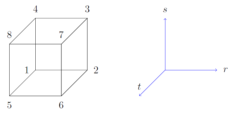

Fig. 1 Geometry description in .rea file (sketch of one element ordering - Preprocessor corner notation)

Curved Sides¶

This section describes the curvature of the elements. It is expressed as deformation of the linear elements. Therefore, if no elements are curved (if only linear elements are present) the section remains empty.

The section header may look like this:
640 Curved sides follow IEDGE,IEL,CURVE(I),I=1,5, CCURVE
Curvature information is provided by edge and element. Therefore up to 12 curvature entries can be present for each element. Only non-trivial curvature data needs to be provided, i.e., edges that correspond to linear elements, since they have no curvature, will have no entry. The formatting for the curvature data is provided in Table 16.

Table 16 Curvature information specification¶

IEDGE IEL CURVE(1) CURVE(2) CURVE(3) CURVE(4) CURVE(5) CCURVE

9 2 0.125713 -0.992067 0.00000 0.00000 0.00000 m

10 38 0.125713 -0.992067 3.00000 0.00000 0.00000 m

1 40 1.00000 0.000000 0.00000 0.00000 0.00000 C

There are several types of possible curvature information represented by CCURVE. This include:

‘C’ stands for circle and is given by the radius of the circle, in CURVE(1), all other compoentns of the CURVE array are not used but need to be present.

‘s’ stands for sphere and is given by the radius and the center of the sphere, thus filling the first 4 components of the CURVE array. The fifth component needs to be present but is not utilized.

‘m’ is given by the coordinates of the midside-node, thus using the first 3 components of the CURVE array, and leads to a second order reconstruction of the face. The fourth and fifth components need to be present but are not utilized.

Both ‘C’ and ‘s’ types allow for a surface of as high order as the polynomial used in the spectral method, since they have an underlying analytical description, any circle arc can be fully determined by the radius and end points. However for the ‘m’ curved element descriptor the surface can be reconstructed only up to second order. This can be later updated to match the high-order polynomial after the GLL points have been distributed across the boundaries. This is the only general mean to describe curvature currrently in Nek5000 and corresponds to a HEX20 representation.

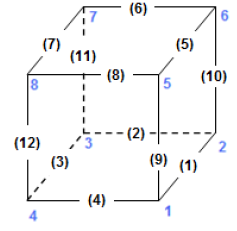
Fig. 2 Edge numbering in .rea file, the edge number is in between parenthesis. The other numbers represent vertices.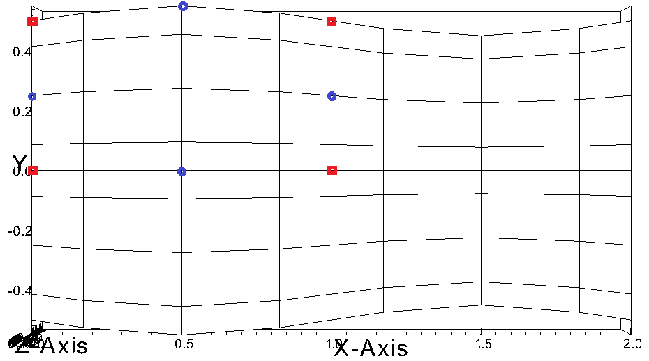

Fig. 3 Example mesh - with curvature. Circular dots represent example midsize points.

Boundaries¶

Boundaries are specified for each field in sequence: velocity, temperature and passive scalars. The section header for each field will be as follows (example for the velocity):
***** FLUID   BOUNDARY CONDITIONS *****
and the data is stored as illustarted in Table 17. For each field boundary conditions are listed for each face of each element.

Boundary conditions are given in order per each element, see Table 17 column IEL, and faces listed in ascending order 1-6 in column IFACE. Note that the header in Table 17 does not appear in the actual .rea.

The ordering for faces each element is shown in Fig. 4. A total equivalent to $6N_{field}$ boundary conditions are listed for each field, where $N_{field}$ is the number of elements for the specific field. $N_{field}$ is equal to the total number of fluid elements for the velocity and equal to the total number of elements (including solid elements) for temperature. For the passive scalars it will depend on the specific choice, but typically scalars are solved on the temeprature mesh (solid+fluid).

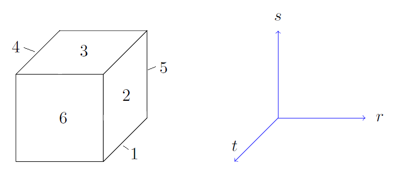
Fig. 4 Face ordering for each element.

Each BC letter condition is formed by three characters. Common BCs include:

E - internal boundary condition. No additional information needs to be provided.

SYM - symmetry boundary condition. No additional information needs to be provided.

P - periodic boundary conditions, which indicates that an element face is connected to another element to establish a periodic BC. The connecting element and face need be to specified in CONN-IEL and CONN-IFACE.

v - imposed velocity boundary conditions (inlet). The value is specified in the user subroutines. No additional information needs to be provided in the .rea file.

W - wall boundary condition (no-slip) for the velocity. No additional information needs to be provided.

O - outlet boundary condition (velocity). No additional information needs to be provided.

t - imposed temperature boundary conditions (inlet). The value is specified in the user subroutines. No additional information needs to be provided in the .rea file.

f - imposed heat flux boundary conditions (temperature). The value is specified in the user subroutines. No additional information needs to be provided in the .rea file.

I - adiabatic boundary conditions (temeperature). No additional information needs to be provided.

Many of the BCs support either a constant specification or a user defined specification which may be an arbitrary function. For example, a constant Dirichlet BC for velocity is specified by V, while a user defined BC is specified by v. This upper/lower-case distinction is used for all cases. There are about 70 different types of boundary conditions in all, including free-surface, moving boundary, heat flux, convective cooling, etc. The above cases are just the most used types.

Table 17 Formatting of boundary conditions input.¶

CBC IEL IFACE CONN-IEL CONN-IFACE

E 1 1 4.00000 3.00000 0.00000 0.00000 0.00000

.. .. .. .. .. .. .. ..

W 5 3 0.00000 0.00000 0.00000 0.00000 0.00000

.. .. .. .. .. .. .. ..

P 23 5 149.000 6.00000 0.00000 0.00000 0.00000

SIZE¶

SIZE file defines the problem size, i.e.the spatial points at which the solution is to be evaluated within each element, number of elements per processor etc. The SIZE file governs the memory allocation for most of the arrays in Nek5000, with the exception of those required by the C utilities. The basic parameters of interest in SIZE are:

ldim = 2 or 3. This must be set to 2 for two-dimensional or axisymmetric simulations (the latter only partially supported) or to 3 for three-dimensional simulations.
lx1 controls the polynomial order of the solution, $N =$ lx1 $-1$.
lxd controls the polynomial order of the (over-)integration/dealiasing. Strictly speaking ${\tt lxd=3 * lx1/2}$ is required but often smaller values are good enough.
lx2 = lx1 or lx1-2 and is an approximation order for pressure that determines the formulation for the Navier-Stokes solver (i.e., the choice between the $\mathbb{P}_N - \mathbb{P}_N$ or $\mathbb{P}_N - \mathbb{P}_{N-2}$ spectral-element methods).
lelg, an upper bound on the total number of elements in your mesh.
lpmax, a maximum number of processors that can be used (Deprecated as of the latest master branch)
lpmin, a minimum number of processors that can be used
ldimt, an upper bound on a number of auxilary fields to solve (temperature + other scalars, minimum is 1).

The optional upper bounds on parameters in SIZE are (minimum being 1 unless otherwise noted):

lhis, a maximum history (i.e. monitoring) points.
maxobj, a maximum number of objects.
lpert, a maximum perturbations.
toteq, a maximum number of conserved scalars in CMT (minimum could be 0).
nsessmax, a maximum number of (ensemble-average) sessions.
lxo, a maximum number of points per element for field file output (lxo $\geq$ lx1).
lelx, lely, lelz, a maximum number of element in each direction for global tensor product solver and/or dimentions.
mxprev, a maximum dimension of projection space (e.g. 20).
lgmres, a maximum dimension of Krylov space (e.g. 30).
lorder, a maximum order of temporal discretization (minimum is2 see also characteristic/OIFS method).
lelt determines the maximum number of elements per processor (should be not smaller than nelgt/lpmin, e.g. lelg/lpmin+1) (promoted to basic section as of the latest master branch).
lx1m, a polynomial order for mesh solver that should be equal to lx1 in case of ALE and in case of stress-formulation (=1 otherwise).
lbelt determines the maximum number of elements per processor for MHD solver that should be equalt to lelt (=1 otherwise).
lpelt determines the maximum number of elements per processor for linear stability solver that should be equalt to lelt (=1 otherwise).
lcvelt determines the maximum number of elements per processor for CVODE solver that should be equalt to lelt (=1 otherwise).
lfdm equals to 1 for global tensor product solver (that uses fast diagonalization method) being 0 otherwise.

Note that one also need to include the following line to SIZE file:

include 'SIZE.inc'

that defines addional internal parameters.

Mesh Partitioning File (.map/.ma2)¶

TODO: Add more details

Restart/Output files (.f#####)¶

Field files are used to read/write physical fields in both serial and parallel. They have extension .f##### where # is a numeral. The file format is unique to Nek5000 and is described in this section.

The file is composed of:

Header

Global element IDs, coordinates, and field data

Metadata

The header provides information about the types, sizes, and layout of the field data. The header is a fixed size of 132 bytes. Its data elements are encoded as either ASCII or binary values. In the table below, the offsets and widths are measured in bytes. Note that consecutive entries are separated by a single byte, which is the ASCII space character. Finally, note that the data entries do not require all 132 bytes.

Some elements that require additional explanation are:

nz: This is the number of GLL gridpoints in the z-direction. If equal to 1, the field data were produced for a 2D simulation. If > 1, the data were produced for a 3D simulation.
rdcode: Specifies the type and ordering of fields that are present in this file. The code can consist of the following. All fields are optional, but if present, they are expected to appear in this order.
- X : Coordinates
- U : Velocity
- P : Pressure
- T : Temperature
- S#: Passive scalar(s). # is a numeral that specifies the number of different passive scalars.
test value: When Nek5000 writes the header to file, it writes the specific value 6.54321 as a test value. When the file is later read – possibly on a different computer – the test value is read and compared to the expected value. If the values match, then the computer that wrote the file and the computer that is now reading the file use the same endianness for floating-point numbers. If not, the computers have different endianness. In that case, the floating-point data should be byte-swapped by the computer reading the data.

Name	Offset	Width	Encoding	Datatype	Description
`tag`	0	4	ASCII	text	The string `#std`. Tags the start of the fil
`wdsize`	5	1	ASCII	integer	Floating-point precision of field data (in bytes)
`nx`	7	2	ASCII	integer	Number of GLL points per element in x direction
`ny`	10	2	ASCII	integer	Number of GLL points per element in y direction
`nz`	13	2	ASCII	integer	Number of GLL points per element in z direction
`nelt`	16	10	ASCII	integer	Number of elements in this file
`nelgt`	27	10	ASCII	integer	Number of global elements
`time`	38	20	ASCII	decimal	Absolute simulation time of this file’s state
`iostep`	59	9	ASCII	integer	I/O timestep of this file’s state
`fid`	69	6	ASCII	integer	Index of this file (when using multi-file output)
`nfileoo`	76	6	ASCII	integer	Number of files produced at this I/O step
`rdcode`	83	10	ASCII	text	Specifies which fields contained in this file
`p0th`	94	15	ASCII	decimal	Thermodynamic pressure
`if_press_mesh`	110	1	ASCII	text	States whether pressure mesh is being used
`test_value`	112	4	binary	32-bit float	The decimal 6.54321. Used to test endianness.

The global element IDs, coordinates, and field data start at offset 136 bytes. Integer data are always 32-bit. The precision of floating-point data is inferred from the value of wdsize (see above). The number of dimensions (ndims) is inferred from nz (see above). The global element IDs are required, but the coordinates and any field data are optional. Their presence of coordinates and field data are inferred from rdcode, as described above.

Value	Datatype	Shape
Global element IDs	integer	`(nelt)`
Coordinates	float	`(nelt, ndims, nx * ny * nz)`
Velocity	float	`(nelt, ndims, nx * ny * nz)`
Pressure	float	`(nelt, nx * ny * nz)`
Temperature	float	`(nelt, nx * ny * nz)`
Passive scalars	float	`(nscalars, nelt, nx * ny * nz)`

TODO: Describe metadata