Stabilizing Filters
Nek5000 includes two options to implement a stabilizing filter. Both methods will drain energy from the solution at the lowest resolved wavelengths, effectively acting as a sub-grid scale dissipation model. A filter is necessary to run an LES turbulence model in Nek5000 and spectral methods in general, as they lack the numerical dissipation necessary to stabilize a so-called “implicit LES” method, which relies on a lack of resolution to provide dissipation. Both methods described here demonstrate spectral convergence for increasing polynomial order as they use the same underlying convolution operator, but apply it in different ways.
The convolution operator is applied on an element-by-element basis. Functions in the SEM are locally represented on each element as \(N^{th}\)-order tensor-product Lagrange polynomials in the reference element, \(\hat\Omega\equiv[-1,1]^3\). This representation can readily be expressed as a tensor-product of Legendre polynomials, \(P_k\). For example, consider
| Reminder: | \(N\) is the polynomial order, \(N=\) lx1 \(-1\) (See the SIZE file) |
|---|
where \(u(x)\) is any polynomial of degree \(N\) on \([-1,1]\). As each Legendre polynomial corresponds to a wavelength on \([-1,1]\), a filtered variant of \(u(x)\) can be constructed from
By choosing appropriate values for the weighting factors, \(\sigma_k\), we can control the characteristics of the filter. In Nek5000 we select a filter cutoff ratio, \((N'+1)/(N+1)\), which can also be equivalently expressed as a number of filtered modes, \(N_{modes}=N-N'\). Weights are chosen as
to construct a low-pass filter. An example is shown below in Fig. 5. The signal produced by this filter would have the highest Legendre mode (shortest wavelength) completely removed with the next two highest modes significantly diminished. However, if the energy of the input signal is fully resolved on the first six modes, the filter would not affect the signal at all.
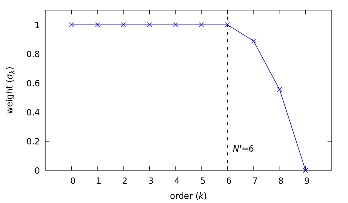
Fig. 5 Example of a strong low-pass filter.
To construct the filter on a three-dimensional element, we define \(F\) as the matrix operation that applies for this one-dimensional low-pass filter. From there, the convolution operator representing the three-dimensional low-pass filter, \((G*)\), on the reference element, \(\hat\Omega\), is given by the Kronecker product \(F \otimes F \otimes F\)
Warning
The filtered wavelengths depend on the local element size, so the filtering operation is NOT necessarily uniform across the domain.
Explicit Filter
The explicit filter is based on a method described by Fischer and Mullen [Fischer2001]. It is so named as it applies a low-pass filtering operation directly to all the solution variables at the end of every time step, explicitly filtering the solution. In the turbulence energy cascade, energy is transferred from large scales to lower scales. In methods with negligible numerical dissipation, such as the SEM, this energy builds in the lowest resolved length-scales, or shortest resolved wavelengths. By applying a low-pass filter, Nek5000 removes energy from the shortest wavelengths, acting as a sub-grid dissipation model and stabilizing the solution.
The explicit filter can be invoked by setting the filtering=explicit key in the [GENERAL] section of the .par file.
The weight is controlled by the filterWeight key and the cutoff ratio is controlled by either the filterCutoffRatio or the filterModes keys.
The filterWeight key controls the weight of the highest filtered mode
Nek5000 will then parabolically decrease the effect of the filter for each subsequent lower mode until \(\sigma_{N'}=1\).
The cutoff ratio can be controlled by the filterCutoffRatio key
The cutoff ratio is assigned as a real, while the corresponding value of \(N'\) is restricted to integer values.
Consequently, Nek5000 will pick a value of \(N'\) to match the specified cutoff ratio as closely as possible.
| Note: | For any non-zero value of filterWeight and filterCutoffRatio\(<1\), Nek5000 will always filter at least 1 mode. |
|---|
It may be more intuitive to directly assign the number of modes with the filterModes key
| Note: | The filterModes key only supports \(N-N'\ge2\). To filter only one mode, use filterCutoffRatio = 0.99. |
|---|
The weights for each mode are printed to the logfile at the end of the first time step. To verify your filter settings, look for the two lines highlighted below. It will have two rows by \((N+1)\) columns. The second row corresponds to the values for \(\sigma_k\), with \(\sigma_0\) on the left and \(\sigma_N\) on the right.
          1  Fluid done  5.5101E+01  4.0337E+00
filt amp 0.0000 0.0000 0.0000 0.0000 0.0000 0.0000 0.0125 0.0500
filt trn 1.0000 1.0000 1.0000 1.0000 1.0000 1.0000 0.9875 0.9500

Step      2, t= 2.0000000E-03, DT= 1.0000000E-03, C=  1.454 4.5714E+00 4.5714E+00
In practice, for an LES turbulence model, we want to use as gentle of a filter as possible while maintaining stability. The filtering method demonstrates spectral convergence, so for stronger settings, the LES solution will still converge in the limit of increasing polynomial order. However, a strong filter decreases the effective resolution. To take advantage of the full resolution that’s available, the impact of the filter should be minimized. Generally recommended settings for \(N\ge5\) are as follows:
[GENERAL]
filtering = explicit
filterModes = 2
filterWeight = 0.05
This will set up a low-pass filter that touches the two highest Legendre modes and decreases the amplitude of the highest mode by 5%. The weights for this filter are shown below in Fig. 6 for a 7th-order case.

Fig. 6 Weighting for the recommend explicit LES filter
Note
The explicit filter is applied after every time step, consequently its strength is inversely proportional to time step size for marginally resolved cases.
High-Pass Filter
The high-pass filter in Nek5000 is based on a method described by Stolz, Schlatter, and Kleiser [Stolz2005]. It is another method of applying sub-grid scale dissipation. In the high-pass filter method, the convolution operator described above is used to obtain a low-pass filtered signal. The high-pass filter term is then constructed from the difference between the original signal and the low-pass filtered signal. For any scalar, this term has the form
where \(u\) is the original signal, \(\tilde u = G*u\) is the low-pass filtered signal, and \(\chi\) is a proportionality constant. In polynomial space, this term is only non-zero for the last few Legendre modes, \(k>N'\). It is subtracted from the RHS of the momentum, energy, and scalar transport equations, respectively
and acts to provide the necessary drain of energy out of the discretized system.
The high-pass filter can be invoked by setting the filtering=hpfrt key in the [GENERAL] section of the .par file.
The cutoff ratio used in the convolution operator, \((G*)\), is controlled by either the filterCutoffRatio or the filterModes keys, identically to the explicit filter.
The convolution operation used to construct the filtered signal, \(\tilde u\), completely removes the highest Legendre mode \(\sigma_N = 0\). The coefficients for the subsequent lower modes decrease parabolically until \(\sigma_{N'}=1\). This corresponds to a strong low-pass filtering operation, similar to the one shown in Fig. 5.
The overall strength of the high-pass filter is controlled by the proportionality coefficient, \(\chi\), which is set using the filterWeight key.
Typical values for this are \(5\le\chi\le10\), which drains adequate energy to stabilize the simulations.
The high-wavenumber relaxation of the high-pass filter model is similar to the approximate deconvolution approach [Stolz2001]. It is attractive in that it can be tailored to directly act on marginally resolved modes at the grid scale. The approach allows good prediction of transitional and turbulent flows with minimal sensitivity for model coefficients [Schlatter2006]. Furthermore, the high-pass filters enable the computation of the structure function in the filtered or HPF structure-function model in all spatial directions even for inhomogeneous flows, removing the arbitrariness of special treatment of selected (e.g. wall-normal) directions.
Generally recommended settings are as follows
[GENERAL]
filtering = hpfrt
filterModes = 2
filterWeight = 5.0