Overlapping Overset Grids
This tutorial will describe how to run a case with two overlapping meshes (NekNek) from scratch. We illustrate this by using the Periodic Hill case. If you are not familiar with Nek5000, we strongly recommend you begin with the periodic hill tutorial first!
The three key steps to running a case with NekNek are:
- Setting up the mesh with appropriate boundary conditions for the overlapping interface.
- Specifying parameters to control stability and accuracy for the overlapping-Schwarz iterations.
- Modifying
userbcto read Dirichlet boundary data for the overlapping interfaces.
Pre-processing
The pre-processing steps for a NekNek calculation differ from a mono-domain Nek5000 calculation only in terms of ensuring that the appropriate boundary condition int is specified at the overlapping interface.
This boundary condition serves as the flag to let the solver know that Dirichlet data for these boundary conditions must come from interpolation of the data in the overlapping mesh.
Mesh generation
In this tutorial, we generate two meshes to span the entire domain, an upper and a lower mesh.
The lower mesh is generated by genbox with the following input file:
-2                     spatial dimension (will create box.re2)
1                      number of fields
#
#    comments: two dimensional periodic hill
#
#========================================================
#
Box
-22 5                                     Nelx  Nely
0.0 9.0 1.                                x0 x1 ratio
0.0 0.1 0.25 0.5 1.5 2.5                  y0 y1 ratio
P  ,P  ,W  ,int                           BC's:  (cbx0, cbx1, cby0, cby1)
and the upper mesh is generated by genbox with the following input file:
-2 spatial dimension (will create box.re2)
1                      number of fields
#
#    comments: two dimensional periodic hill
#
#========================================================
#
Box
-21 3                 Nelx  Nely
0.0 9.0 1.            x0 x1 ratio
2.25 2.75 2.9 3.0     y0 y1 ratio
P  ,P  ,int,W         BC's:  (cbx0, cbx1, cby0, cby1)
Note: the lower domain spans \(y \in [0,2.5]\) and the upper domain spans \(y \in [2.25,3]\). We also use int for the boundary surfaces that overlap the other domain.
Now the meshes can be generated by running genbox for each of these cases to obtain upper.re2 and lower.re2.
$ genbox <<< upper.box
$ mv box.re2 upper.re2
$ genbox <<< lower.box
$ mv box.re2 upper.re2
| Reminder: | genbox produces a file named box.re2, so you will need to rename the files between generating the separate parts. |
|---|
Once we have both upper and lower mesh files, we need to run genmap for both meshes.
$ genmap
On input specify lower as your casename and press enter to use the default tolerance.
This step will produce lower.ma2 which needs to be generated only once.
Next do the same for the upper mesh to generate upper.ma2.
usr file
As for the mono-domain periodic hill case, we start by copying the template to our case directory:
$ cp $HOME/Nek5000/core/zero.usr hillnn.usr
Modify mesh and add forcing to the flow
As for the mono-domain periodic hill case, we modify the mesh in usrdat2 as:
      subroutine usrdat2()
      implicit none
      include 'SIZE'
      include 'TOTAL'

      integer ntot,i
      real A,B,C,xx,yy,argx,A1

      ntot = lx1*ly1*lz1*nelt

      A   = 4.5
      B   = 3.5
      C   = 1./6.

      do i=1,ntot
         xx   = xm1(i,1,1,1)
         yy   = ym1(i,1,1,1)
         argx = B*(abs(xx-A)-B)
         A1   = C + C*tanh(argx)
         ym1(i,1,1,1) = yy + (3-yy)*A1
      enddo

      return
      end
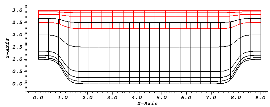
Fig. 21 Modified box mesh graded
Currently, applying a constant mass flux with param(54) and param(55) is not supported with overlapping overset grids.
For this case, we drive the flow using a constant acceleration term in userf as:
      subroutine userf(ix,iy,iz,eg) ! set acceleration term
c
c     Note: this is an acceleration term, NOT a force!
c     Thus, ffx will subsequently be multiplied by rho(x,t).
c
      implicit none
      include 'SIZE'
      include 'TOTAL'
      include 'NEKUSE'

      integer ix,iy,iz,eg,e

c     e = gllel(eg)

      ffx = 0.052
      ffy = 0.0
      ffz = 0.0

      return
      end
Specify NekNek parameters
In usrdat, we specify the number of Schwarz-like iterations and extrapolation order for the boundary conditions of the overlapping interface.
These parameters impact the stability and accuracy of the calculation.
This is done as:
      subroutine usrdat()   ! This routine to modify element vertices
      implicit none
      include 'SIZE'
      include 'TOTAL'

      ngeom  = 5
      ninter = 2

      return
      end
Here we do 4 sub-iterations, ngeom=5, at each time-step between the two meshes, and the temporal extrapolation order, ninter, is 2.
Boundary and initial conditions
The next step is to specify the initial conditions.
This can be done in the subroutine useric as follows:
      subroutine useric(ix,iy,iz,ieg)
      implicit none
      include 'SIZE'
      include 'TOTAL'
      include 'NEKUSE'

      integer ix,iy,iz,ieg

      ux   = 1.0
      uy   = 0.0
      uz   = 0.0
      temp = 0.0

      return
      end
Next we modify userbc to read the boundary conditions, interpolated from overlapping domains, as follows:
      subroutine userbc(ix,iy,iz,iside,eg) ! set up boundary conditions
c
c     NOTE ::: This subroutine MAY NOT be called by every process
c
      implicit none
      include 'SIZE'
      include 'TOTAL'
      include 'NEKUSE'
      include 'NEKNEK'

      integer ix,iy,iz,iside,eg,ie

c      if (cbc(iside,gllel(eg),ifield).eq.'v01')

      ie = gllel(eg)

      if (imask(ix,iy,iz,ie).eq.0) then
        ux   = 0.0
        uy   = 0.0
        uz   = 0.0
        temp = 0.0
      else
        ux = valint(ix,iy,iz,ie,1)
        uy = valint(ix,iy,iz,ie,2)
        uz = valint(ix,iy,iz,ie,3)
        if (nfld_neknek.gt.3) temp = valint(ix,iy,iz,ie,ldim+2)
      endif

      return
      end
Control parameters
The control parameters for this case are the same as that for the mono-domain periodic hill case.
Create two files called lower.par and upper.par, and type in each the following:
# Nek5000 parameter file
[GENERAL]
stopAt = endTime
endTime  = 200

variableDT = yes
targetCFL = 0.4
timeStepper = bdf2

writeControl = runTime
writeInterval = 20

[PROBLEMTYPE]
equation = incompNS

[PRESSURE]
residualTol = 1e-5
residualProj = yes

[VELOCITY]
residualTol = 1e-8
density = 1
viscosity = -100
SIZE file
The static memory layout of Nek5000 requires the user to set some solver parameters through a so called SIZE file.
Typically it’s a good idea to start from our template.
Copy the SIZE.template file from the core directory and rename it SIZE in the working directory:
$ cp $HOME/Nek5000/core/SIZE.template SIZE
For NekNek, the parameter choices are not as straightforward as for a regular case.
Because the two cases are being run from a single executable, the SIZE file must be able to accommodate both cases.
This can be accomplished by “brute force” by picking lelg for the larger of the two cases, lpmin for the smaller of the two and leaving lelt alone.
However, for many practical cases, the two domains may not be of similar size and we may run out of memory, resulting in truncation errors at compile time (see here).
This can be overcome by setting lelt manually and preserving the ratio of number of elements, \(E\), to the number of MPI-ranks, \(L\).
If we have \(L_{tot}\) MPI-ranks (CPU-cores) available, we might choose
We then pick the largest mesh size for lelg, and the smallest rank count for lpmin
Assuming we have 8 MPI-ranks available for this case, that gives lelg=110, lpmin = 3, and lelt=25.
Then, adjust the parameters in the BASIC section
      ! BASIC
      parameter (ldim=2)               ! domain dimension (2 or 3)
      parameter (lx1=8)                ! GLL points per element along each direction
      parameter (lxd=12)               ! GL  points for over-integration (dealiasing)
      parameter (lx2=lx1-0)            ! GLL points for pressure (lx1 or lx1-2)

      parameter (lelg=110)             ! max number of global elements
      parameter (lpmin=3)              ! min number of MPI ranks
      parameter (lelt=25)              ! max number of local elements per MPI rank
      parameter (ldimt=1)              ! max auxiliary fields (temperature + scalars)
and in the OPTIONAL section, set the maximum number of sessions, nsessmax to 2
      ! OPTIONAL
      parameter (ldimt_proj=1)         ! max auxiliary fields residual projection
      parameter (lelr=lelt)            ! max number of local elements per restart file
      parameter (lhis=1)               ! max history/monitoring points
      parameter (maxobj=1)             ! max number of objects
      parameter (lpert=1)              ! max number of perturbations
      parameter (nsessmax=2)           ! max sessions to NEKNEK
      parameter (lxo=lx1)              ! max GLL points on output (lxo>=lx1)
      parameter (mxprev=20)            ! max dim of projection space
      parameter (lgmres=30)            ! max dim Krylov space
      parameter (lorder=3)             ! max order in time
      parameter (lx1m=1)               ! GLL points mesh solver
      parameter (lfdm=0)               ! unused
      parameter (lelx=1,lely=1,lelz=1) ! global tensor mesh dimensions
For this tutorial we have set our polynomial order to be \(N=7\) - this is defined in the SIZE file above as lx1=8 which indices that there are 8 points in each spatial dimension of every element.
Additional details on the parameters in the SIZE file are given here.
Compilation
With the hillnn.usr, and SIZE files created, you should now be all set to compile and run your case!
As a final check, you should have the following files:
If for some reason you encountered an insurmountable error and were unable to generate any of the required files, you may use the provided links to download them. After confirming that you have all eight, you are now ready to compile
$ makenek hillnn
If all works properly, upon compilation the executable nek5000 will be generated.
Running the case
Now you are all set, just run
$ neknekb lower upper 5 3
to launch an MPI job on your local machine using 8 ranks.
Post-processing the results
As the case runs, it will produce restart files for both sessions, upper and lower, independently.
You will need to use visnek for both sessions to generate two metadata files.
They can be visualized separately or together by loading both sets into ParaView or VisIt to post-process the results
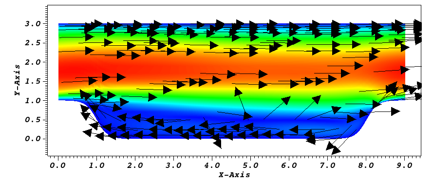
Fig. 22 Steady-State flow field visualized in Visit/Paraview. Vectors represent velocity. Colors represent velocity magnitude. Note, velocity vectors are equal size and not scaled by magnitude.