Fully Developed Laminar Flow¶

In this tutorial we will be building a case that involves incompressible laminar flow in a channel with a constant heat flux applied. This case uses air as a working fluid and will be simulated using fully dimensional quantities. A diagram of the case is provided in Fig. 11 and the necessary case parameters are provided in Table 28. Note that round numbers have been selected for the fluid properties and simulation parameters for the sake of simplicity.

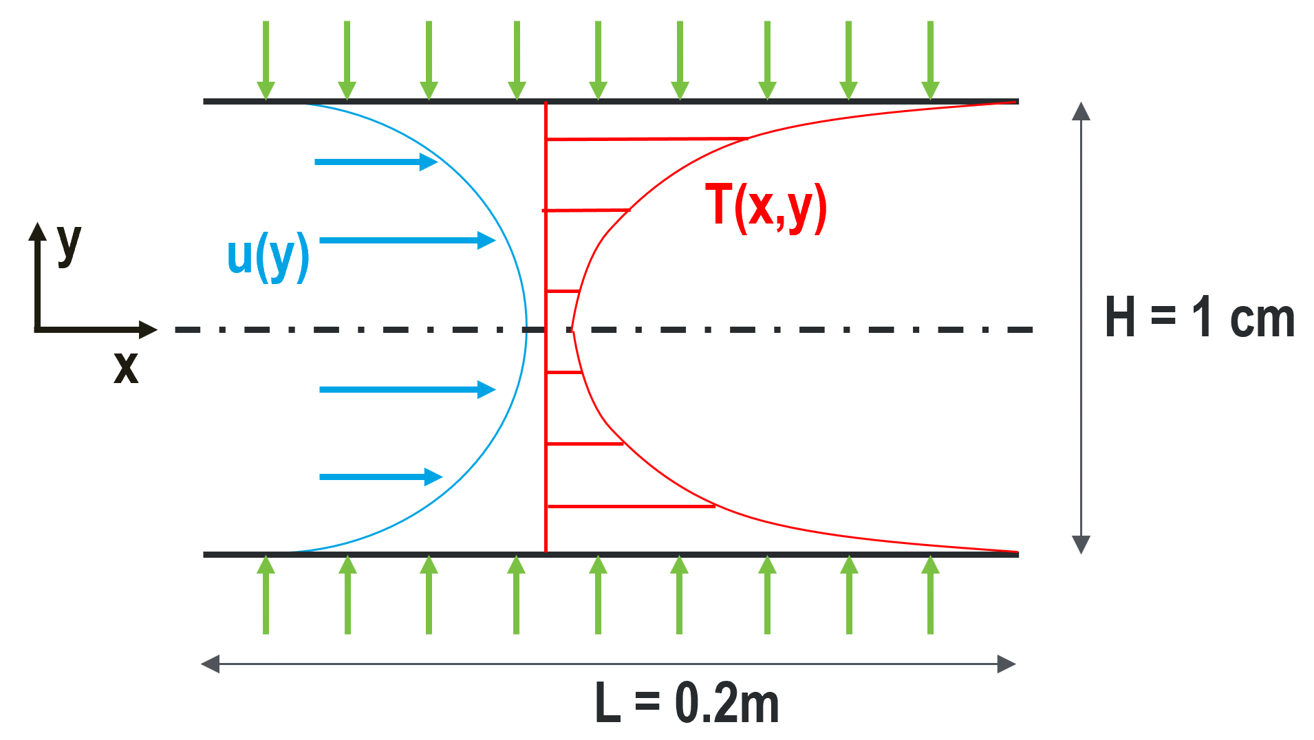
Fig. 11 Diagram describing the case setup for fully developed laminar flow in a channel..

Table 28 Fluid properties and simulation parameters¶
Parameter name	variable	value
channel height	$H$	1 cm
channel length	$L$	20 cm
mean velocity	$U_m$	0.5 m/s
heat flux	$q''$	300 W/m²
inlet temperature	$T_{in}$	10 C
density	$\rho$	1.2 kg/m³
viscosity	$\mu$	0.00002 kg/m-s
thermal conductivity	$\lambda$	0.025 W/m-K
specific heat	$c_p$	1000 J/kg-K

This case has analytic solutions to the momentum and energy equations which makes it easy to confirm if the problem is setup correctly. These expressions will be used to test the accuracy of the solution.

(1)¶\[u(y) = \frac{3}{2} U_m \left( 1 - 4\left(\frac{y}{H}\right)^2\right)\]

(2)¶\[T(x,y)-T_b(x) = \frac{q'' H}{2\lambda}\left( 3\left(\frac{y}{H}\right)^2 - 2\left(\frac{y}{H}\right)^4-\frac{39}{280}\right)\]

where the bulk temperature is given by the expression

\[T_b(x) = \left(\frac{2q''}{U_m \rho c_p H}\right)x + T_{in}\]

Before You Begin¶

This tutorial assumes that you have installed Nek5000 in your home directory and have setup your execution PATH. Before running the case, you will need to compile the tools genbox and genmap. These can be compiled using the following command in the $HOME/Nek5000/tools directory:

$ ./maketools genbox
$ ./maketools genmap

Before building the case, the user should set up a case subdirectory in their run directory.

$ cd $HOME/Nek5000/run
$ mkdir fdlf
$ cd fdlf

Mesh Generation¶

This tutorial uses a simple rectangular box mesh generated by genbox. To create the input file, copy the following script and save the file as fdlf.box.

-2                     spatial dimension (will create box.re2)
2                      number of fields
#
#    comments: periodic laminar flow
#
#========================================================
#
Box                                       fdlf
-50 -5                                    Nelx  Nely
0.0 0.2 1.0                               x0 x1 ratio
0.0 0.005 0.7                             y0 y1 ratio
v  ,O  ,SYM,W                             Velocity BC's:  (cbx0, cbx1, cby0, cby1)
t  ,O  ,I  ,f                             Temperature BC's:  (cbx0, cbx1, cby0, cby1)

For this mesh we are specifying 50 uniform elements in the stream-wise ($x$) direction and 5 uniform elements in the span-wise ($y$) direction. The velocity boundary conditions in the x-direction are a standard Dirichlet velocity boundary condition at $x_{min}$ and an open boundary condition with zero pressure at $x_{max}$. The velocity boundary conditions in the y-direction are a symmetric boundary at $y_{min}$ and a wall with no slip condition at $y_{max}$.. The temperature boundary conditions in the x-direction are a standard Dirichlet boundary condition at $x_{min}$ and an outflow condition with zero gradient at $x_{max}$. The temperature boundary conditions in the y-direction are an insulated condition with zero gradient at $y_{min}$ and a constant heat flux at $y_{max}$. Note that the boundary conditions specified with lower case letters must have values assigned in userbc, which will be shown later in this tutorial. Now we can run genbox with

$ genbox

When prompted provide the input file name, which for this case is fdlf.box. The tool will produce binary mesh and boundary data file box.re2 which should be renamed to fdlf.re2.

Once we have the mesh file, we need to run the domain partitioning tool, genmap.

$ genmap

On input specify fdlf as your casename and press enter to use the default tolerance. This step will produce fdlf.ma2 which contains the element partitioning information. You do not have to specify the number of MPI-ranks you plan to run the case with when you use genmap, as it contains the partitioning for all possible choices.

tip:	If either `genbox` or `genmap` cannot be located by your shell, check to make sure the `Nek5000/tools` directory is in your path. For help see here.

Control parameters¶

The control parameters for any case are given in the .par file. For this case, create a new file called fdlf.par with the following:

#
# nek parameter file
#
[GENERAL]
dt = 1.0e-4
numsteps = 10000
writeInterval = 2000

userParam01 = 0.01   #channel height [m]
userParam02 = 0.5    #mean velocity [m/s]
userParam03 = 300.0  #heat flux [W/m^2]
userParam04 = 10     #inlet temperature [C]

[VELOCITY]
density = 1.2        #kg/m3
viscosity = 0.00002  #kg/m-s

[TEMPERATURE]
rhoCp = 1200.0       #J/m3-K
conductivity = 0.025 #W/m-K

For this case the properties evaluated are for air at ~20 C. Note that rhoCp is the product of density and specific heat. The userParam list represents an easy way of passing data to Nek5000 that can later be used throughout the .usr file. Additionally, like all values specified in the .par file, they can be changed without the need to recompile Nek5000.

The required values for the initial and boundary conditions specified by lower case letters in the .box file are defined here as a list of user given parameters, as well as the height of the channel. These initial and boundary conditions will later be called in respective subroutines of the .usr file.

User Routines File (.usr)¶

The user file implements various subroutines to allow the user to interact with the solver. Note that only the subroutines that need to be edited to run this case will be discussed. The remaining routines can be left as is. For more information on the .usr file and the available subroutines see here.

To get started we copy the template to our case directory

$ cp $HOME/Nek5000/core/zero.usr fdlf.usr

Boundary and initial conditions¶

The boundary conditions can be setup in subroutine userbc as shown below, where the highlighted lines indicate where the actual boundary condition is specified. The velocity and temperature are set to the analytic profiles given by Eqs. (1) and (2) and the heat flux is set to a constant value.

      subroutine userbc(ix,iy,iz,iside,eg) ! set up boundary conditions
c
c     NOTE ::: This subroutine MAY NOT be called by every process
c
      implicit none
      include 'SIZE'
      include 'TOTAL'
      include 'NEKUSE'

      integer ix,iy,iz,iside,eg
      real H,um,qpp,Tin,con,term

c      if (cbc(iside,gllel(eg),ifield).eq.'v01')

      H    = uparam(1)     !channel height
      um   = uparam(2)     !mean velocity
      qpp  = uparam(3)     !heat flux
      Tin  = uparam(4)     !mean inlet temperature
      con  = cpfld(2,1)    !thermal conductivity
      term = qpp*H/(2*con)
      
      ux   = um*3./2.*(1-4.*(y/H)**2)
      uy   = 0.0
      uz   = 0.0
      temp = term*(3.*(y/H)**2-2.*(y/H)**4-39./280.)+Tin
      flux = qpp

      return
      end

The channel height, mean velocity, heat flux, and mean inlet temperature are all called from the list of user defined parameters in the .par file. The thermal conductivity is set from the field coefficient array, which is set from the conductivity specified for the temperature field in the .par file.

The next step is to specify the initial conditions. This can be done in the subroutine useric as shown. Again, the actual inlet condition is specified with the highlighted lines.

      subroutine useric(ix,iy,iz,ieg)
      implicit none
      include 'SIZE'
      include 'TOTAL'
      include 'NEKUSE'
      
      integer ix,iy,iz,ieg
      real um,Tin
      
      um = uparam(2)
      Tin = uparam(4)
      
      ux   = um
      uy   = 0.0
      uz   = 0.0
      temp = Tin
      
      return
      end

As with userbc, the inlet temperature and mean velocity are set from the list of user defined parameters in the .par file.

SIZE file¶

It is recommended to copy a template of the SIZE file from the core directory and rename it SIZE in the working directory:

$ cp $HOME/Nek5000/core/SIZE.template SIZE

Then, in the BASIC section, adjust the domain dimension (ldim) and the max number of global elements (lelg).

      ! BASIC
      parameter (ldim=2)               ! domain dimension (2 or 3)
      parameter (lx1=8)                ! GLL points per element along each direction
      parameter (lxd=12)               ! GL  points for over-integration (dealiasing) 
      parameter (lx2=lx1-0)            ! GLL points for pressure (lx1 or lx1-2)
                                     
      parameter (lelg=250)             ! max number of global elements
      parameter (lpmin=1)              ! min number of MPI ranks 
      parameter (lelt=lelg/lpmin + 3)  ! max number of local elements per MPI rank
      parameter (ldimt=1)              ! max auxiliary fields (temperature + scalars)

For this tutorial we have set our polynomial order to be $N=7$ which is defined in the SIZE file as lx1=8 which indicates that there are 8 points in each spatial dimension of every element. The number of dimensions is specified using ldim and the number of global elements used is specified using lelg.

Compilation¶

You should now be all set to compile and run your case! As a final check, you should have the following files:

fdlf.usr

fdlf.par

fdlf.re2

fdlf.ma2

SIZE

If for some reason you encountered an insurmountable error and were unable to generate any of the required files, you may use the provided links to download them. After confirming that you have all five, you are now ready to compile

$ makenek fdlf

If the compilation is successful, the executable nek5000 will be generated.

Running the case¶

Now you can run the case

$ nekbmpi fdlf 4

To launch an MPI jobs on your local machine using 4 ranks. The output will be redirected to logfile.

Post-processing the results¶

Once execution is completed your directory should now contain 5 checkpoint files that look like this:

fdlf0.f00001
fdlf0.f00002
...

The preferred mode for data visualization and analysis with Nek5000 is to use Visit/ParaView. One can use the script visnek, to be found in /scripts. It is sufficient to run:

$ visnek fdlf

to obtain a file named fdlf.nek5000 which can be recognized in Visit/ParaView. In the viewing window one can visualize the flow-field as depicted in Fig. 12 as well as the temperature profile as depicted in Fig. 13 below.

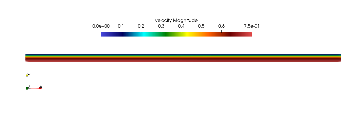
Fig. 12 Steady-State flow field visualized in Visit/ParaView. Colors represent velocity magnitude.

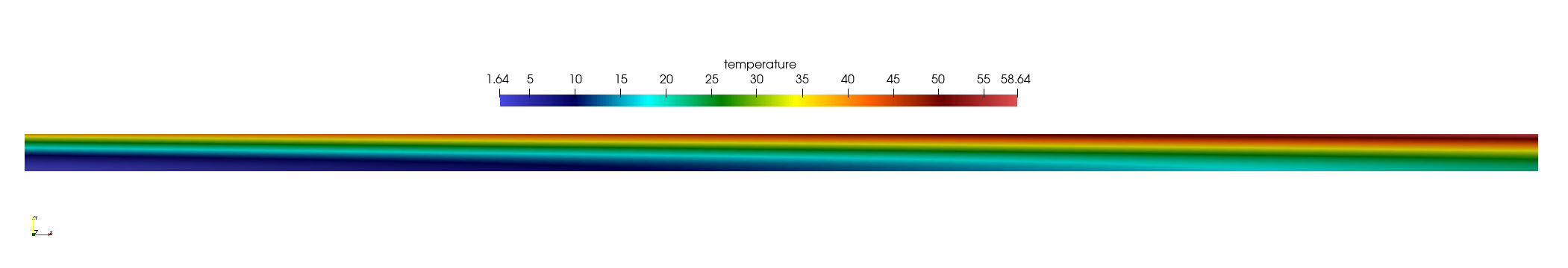
Fig. 13 Temperature profile visualized in Visit/ParaView.

Plots of the velocity and temperature varying along the y-axis as evaluated by Nek5000 compared to the analytic solutions provided by Eqs. (1) and (2) respectively are shown below in Fig. 14 and Fig. 15.

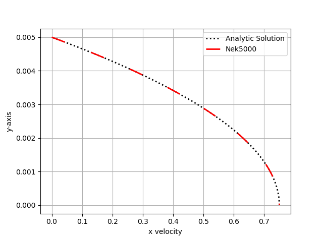
Fig. 14 Nek5000 velocity solutions plotted against analytical solutions.

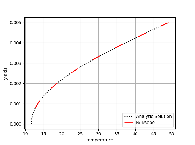
Fig. 15 Nek5000 temperature solutions plotted against analytical solutions.