Periodic Hill
Warning
This tutorial is written for the most recent version of Nek5000 available on GitHub. To view the previous version of this tutorial compatible with V19, see here.
This tutorial will describe how to run a case from scratch. We illustrate this procedure through a relatively simple example involving incompressible laminar flow in a two-dimensional periodic hill domain. Our implementation is loosely based on the case presented by Mellen et al. [Mellen2000]. A thorough review for this case can be found in the ERCOFTAC knowledge base wiki.
Pre-processing
We assume that you have installed Nek5000 in your home directory.
This tutorial requires that you have the tools genbox and genmap compiled.
Make sure $HOME/Nek5000/bin is in your search PATH.
Cases are setup in Nek5000 by editing case files. Users should select an editor of choice with which to do this (e.g vi). A case being simulated involves data for mesh, parameters, etc. As a first step, the user should create a case directory in their run directory.
$ cd $HOME/Nek5000/run
$ mkdir hillp
$ cd hillp
Mesh generation
In this tutorial we use a simple box mesh generated by
genbox with the following input file:
-2                     spatial dimension (will create box.re2)
1                      number of fields
#
#    comments: two dimensional periodic hill
#
#========================================================
#
Box                                       hillp
-22 8                                     Nelx  Nely
0.0 9.0 1.                                x0 x1 ratio
0.0 0.1 0.25 0.5 1.5 2.5 2.75 2.9 3.0     y0 y1 ... y8
P  ,P  ,W  ,W                             BC's:  (cbx0, cbx1, cby0, cby1)
For this mesh we are specifying 22 uniform elements in the stream-wise (x) direction.
8 non-uniform elements are specified in the span-wise (y) direction in order to resolve the boundary layers.
The boundary conditions are periodic in the x-direction and no-slip in the y.
Additional details on generating meshes using genbox can be found here. Now we can run genbox with
$ genbox
On input provide the input file name (e.g. hillp.box).
The tool will produce a binary mesh and boundary data file box.re2 which should be renamed to hillp.re2.
usr file
The user file implements various subroutines to allow the user to interact with the solver.
To get started we copy the template to our case directory
$ cp $HOME/Nek5000/core/zero.usr hillp.usr
Modify mesh
For a periodic hill, we will need to modify the geometry. Let \({\bf x} := (x,y)\) denote the old geometry, and \({\bf x}' := (x',y')\) denote the new geometry. For a domain with \(y\in [0,3]\) and \(x\in [0,9]\) the following function will map the straight pipe geometry to a periodic hill:
where \(A=4.5, B=3.5, C=1/6\). We have chosen these constants so that the height of the hill (our reference length), \(h=1\). Note that, as \(y \longrightarrow 3\), the perturbation, goes to zero. So that near \(y = 3\), the mesh recovers its original form.
In Nek5000, we can specify this through usrdat2 in the .usr file as follows.
The highlighted line shows where the mesh is deformed.
      subroutine usrdat2()
      implicit none
      include 'SIZE'
      include 'TOTAL'

      integer ntot,i
      real A,B,C,xx,yy,argx,A1

      ntot = lx1*ly1*lz1*nelt

      A   = 4.5
      B   = 3.5
      C   = 1./6

      do i=1,ntot
         xx   = xm1(i,1,1,1)
         yy   = ym1(i,1,1,1)
         argx = B*(abs(xx-A)-B)
         A1   = C + C*tanh(argx)
         ym1(i,1,1,1) = yy + (3-yy)*A1
      enddo

      return
      end
By modifying the mesh in usrdat2, the modification is applied to the GLL points directly.
This allows the mesh to conform to the specified profile to \(N^{th}\)-order accuracy.
The deformed mesh with the GLL points is shown in Fig. 16 below.
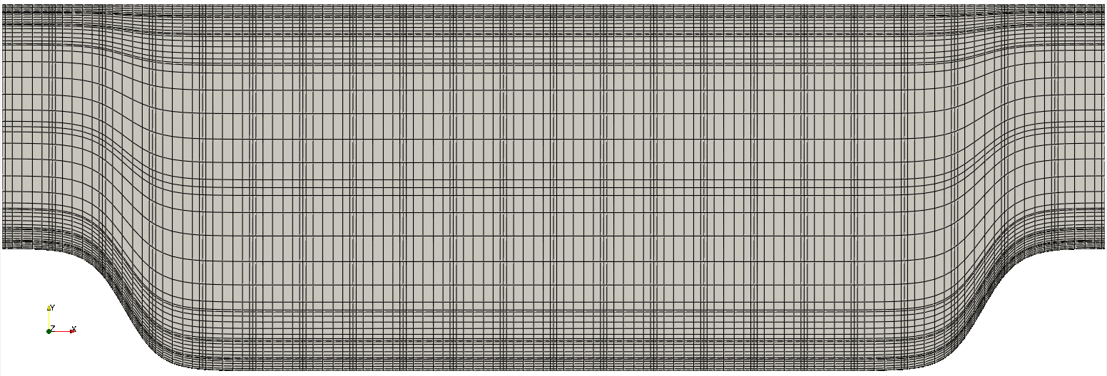
Fig. 16 Modified box mesh graded
Initial & boundary conditions
The next step is to specify the initial conditions.
This can be done in the subroutine useric as follows:
      subroutine useric(ix,iy,iz,ieg)
      implicit none
      include 'SIZE'
      include 'TOTAL'
      include 'NEKUSE'

      integer ix,iy,iz,ieg

      ux   = 1.0
      uy   = 0.0
      uz   = 0.0
      temp = 0.0

      return
      end
For walls and periodic boundaries, nothing needs to be specified in the user file, so userbc can remain unmodified.
Control parameters
The control parameters for any case are given in the .par file.
For this case, using any text editor, create a new file called hillp.par and type in the following
# Nek5000 parameter file
[GENERAL]
stopAt = endTime
endTime  = 200
variableDT = yes
targetCFL = 0.4
writeControl = runTime
writeInterval = 20
constFlowRate = X
meanVelocity = 1.0

[PROBLEMTYPE]
equation = incompNS

[PRESSURE]
residualTol = 1e-5
residualProj = yes

[VELOCITY]
residualTol = 1e-8
density = 1
viscosity = -100
We have set the calculation to stop at the physical time of \(T=200\) (endTime=200) which is roughly 22 flow-thru time units (based on the bulk velocity \(u_b\) and length of periodic pitch, \(L=9\)).
To drive the flow, a forced flow rate in the x-direction is applied such that bulk velocity \(u_b=1\). This is accomplished with the two highlighted lines.
Warning
The forced flow rate options are only intended for use with periodic boundaries!
In choosing viscosity = -100 we are actually setting the Reynolds number. This assumes that
\(\rho \times u_b \times h = 1\) where \(u_b\) denotes the bulk velocity and \(h\) the hill height.
Additional details on the names of keys in the .par file can be found here.
SIZE file
The static memory layout of Nek5000 requires the user to set some solver parameters through a so called SIZE file.
Typically it’s a good idea to start from our template.
Copy the SIZE.template file from the core directory and rename it SIZE in the working directory:
$ cp $HOME/Nek5000/core/SIZE.template SIZE
Then, adjust the following parameters in the BASIC section
      ! BASIC
      parameter (ldim=2)               ! domain dimension (2 or 3)
      parameter (lx1=8)                ! GLL points per element along each direction
      parameter (lxd=12)               ! GL  points for over-integration (dealiasing)
      parameter (lx2=lx1-0)            ! GLL points for pressure (lx1 or lx1-2)

      parameter (lelg=22*8)            ! max number of global elements
      parameter (lpmin=1)              ! min number of MPI ranks
      parameter (lelt=lelg/lpmin + 3)  ! max number of local elements per MPI rank
      parameter (ldimt=1)              ! max auxiliary fields (temperature + scalars)
For this tutorial we have set our polynomial order to be \(N=7\) - this is defined in the SIZE file above as lx1=8 which indices that there are 8 points in each spatial dimension of every element.
Additional details on the parameters in the SIZE file are given here.
Compilation
With the hillp.usr, and SIZE files created, you should now be all set to compile and run your case!
As a final check, you should have the following files:
If for some reason you encountered an insurmountable error and were unable to generate any of the required files, you may use the provided links to download them. After confirming that you have all five, you are now ready to compile
$ makenek hillp
If all works properly, upon compilation the executable nek5000 will be generated.
Running the case
First we need to run our domain paritioning tool
$ genmap
On input specify hillp as your casename and press enter to use the default tolerance. This step will produce hillp.ma2 which needs to be generated only once.
Now you are all set, just run
$ nekbmpi hillp 4
to launch an MPI jobs on your local machine using 4 ranks. The output will be redirected to logfile.
Post-processing the results
Once execution is completed your directory should now contain multiple checkpoint files that look like this:
hillp.f00001
hillp.f00002
...
The preferred mode for data visualization and analysis with Nek5000 is
to use Visit/Paraview. One can use the script visnek, to be found in /scripts. It is sufficent to run
$ visnek hillp
(or the name of your session) to obatain a file named hillp.nek5000 which can be recognized in Visit/Paraview.
In the viewing window one can visualize the flow-field as depicted in Fig. 17.
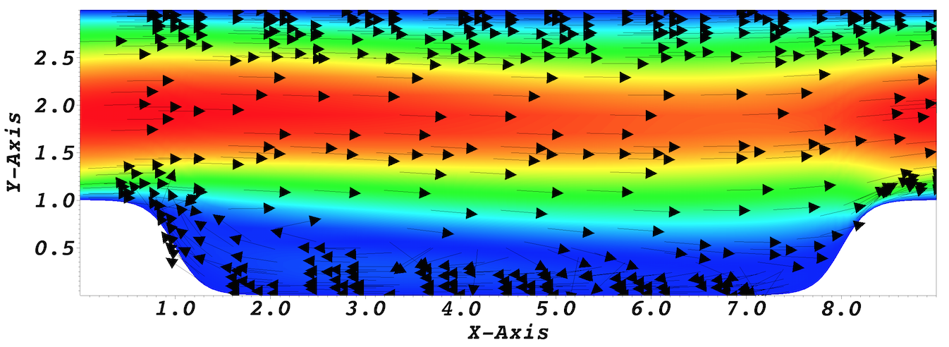
Fig. 17 Visualization of the steady-state flow field. Vectors represent velocity. Colors represent velocity magnitude. Note, velocity vectors are equal size and not scaled by magnitude.