Conjugate Heat Transfer
In this tutorial, we want to simulate a simple 2D Rayleigh-Benard convection (RBC) flow using Nek5000’s conjugate heat transfer capability. The conjugate heat transfer capability solves the energy equation across both solid and liquid subdomains. in the case of RBC, this provides a continuous temperature profile through horizontal walls of finite thickness. The modeled case corresponds to a simplified version of simulations performed by Foroozhani et al. [Foroozani2021].
If you are not familiar with Nek5000, we strongly recommend that you begin with the periodic hill example first! Similarly, we start by generating a 2D mesh, and modify the case files for this instance afterwards and finally run the case.
Pre-processing
Users must always bear in mind, when setting up a test case in Nek5000, case files will need to be edited.
Some samples can be found in the Nek5000/examples directory included with the release version.
Note that the examples directory is linked in the github repository as a submodule and can alternatively be obtained here.
Blank template files for the user file, zero.usr, and the SIZE file, SIZE.template, can be found in the Nek5000/core directory.
As a first step, the user should create a case directory in the corresponding run directory:
$ cd $HOME/Nek5000/run
$ mkdir conj_ht
$ cd conj_ht
and copy the template files into this directory.
Additionally, this tutorial requires the ray0.rea file from the Rayleigh-Bernard example found in Nek5000/examples/rayleigh.
We begin by creating the mesh with appropriate bounday conditions and then setting up the parameters and case files.
Mesh generation
This tutorial requires that you have the tools genbox, genmap, reatore2 and preNek compiled.
Note that preNek requires the use of an xterminal.
Make sure the tools directory (typically Nek5000/bin) is in your environment PATH.
Before beginning, it is important to understand that there are two types of mesh topology: the “v-mesh” for the velocity and the “t-mesh” which can be used for the temperature and passive scalars.
The v-mesh (fluid subdomain) is always a subset of the t-mesh and the global element ID numbers of the v-mesh must preceed those of the t-mesh.
Therefore, we generate a v-mesh and t-mesh with appropriate BCs separately and later merge both subdomains using the conjugate heat transfer merge option in preNek.
This ensures the proper element ordering.
First, we create the mesh for the fluid part by creating the following input file in any text editor and running genbox.
Note that any line beginning with ‘#’ is a comment and is ignored by genbox
ray0.rea
2        spatial dimension
2        number of fields
#========================================================
#
#    Example of 2D  .box file for fluid. This gives 2 x 1
#    box with 20 x 10 elements
#
#    If nelx (y or z) < 0, then genbox automatically generates the
#    grid spacing in the x (y or z) direction
#    with a geometric ratio given by "ratio".
#    ( ratio=1 implies uniform spacing )
#
#========================================================
#
Box
-20     -10         nelx,nely,nelz for Box
0.0    2.0   1.0    x0 x1 ratio
0.0    1.0   1.0    y0 y1 ratio
W  ,W  ,W  ,W  ,    V bc's  ! NB:  3 characters each !
I  ,I  ,E  ,E  ,    T bc's  !      You must have 2 spaces!
In this example, the elements are distributed uniformly in the stream-wise (x) and span-wise (y) directions.
All surfaces of the fluid domain are assumed to be wall boundaries, as indicated by 'W '.
The lateral surfaces of the inner domain and solid walls are assumed to be adiabatic, denoted by 'I '.
The thermal boundary conditions for the upper and lower face should be 'E ', which indicates that they are interior boundaries.
This condition is not mandatory, as any boundary condition set on these faces will be overwritten by preNek when the solid and fluid domains are merged with preNek.
However, it is HIGHLY RECOMMENDED to assign any expected interior faces as 'E ', as any unjoined interior boundaries will be caught later by preNek.
This is useful for identifying inconsistencies in mesh generation.
When genbox is run, the tool will produce a file named box.rea containing mesh, boundary condition, and simulation parameter information, which should be renamed to fluid.rea.
In the next step, we create the upper and lower solid parts of finite thickness h=0.2. The lower domain spans \(y \in [-0.2,0]\) and the upper domain spans \(y \in [1,1.2]\).
Note: It is important to keep the number of elements equal in the spanwise direction for different parts. This is to ensure that all the subdomains are conformal on their interfaces.
Both domains can be generated simultaneously by genbox with the following input file:
ray0.rea
2        spatial dimension
2        number of fields
#========================================================
#
#    This gives a 2 x 1 box with 20 x 5 elements
#    here used for Rayleigh Benard convection.
#
#    Note that spatial dimension > 0 implies that box.rea
#    will be ascii, requiring the ray0.rea template.
#
#========================================================
#
Box
-20    -5           nelx,nely,nelz for Box
0.0    2.0   1.0    x0 x1 ratio
-0.2   0.0   1.0    y0 y1 ratio
   ,   ,   ,   ,    V bc's  ! NB:  3 characters each, in order: -x, +x, -y, +y, (-z, +z)!
I  ,I  ,t  ,E  ,    T bc's  !      You must have 2 spaces!!
Box
-20    -5           nelx,nely,nelz for Box
0.0    2.0   1.0    x0 x1 ratio
1.0    1.2   1.0    y0 y1 ratio
   ,   ,   ,   ,    V bc's  ! NB:  3 characters each, in order: left, right, bottom, top
I  ,I  ,E  ,t  ,    T bc's  !      You must have 2 spaces!!
There are a few things worth notice here.
First, no boundary conditions were given for the velocity.
As the generated mesh corresponds only to the solid domain, any provided BCs will be ignored by Nek5000 at runtime and these are left as blank, ' ', to indicate that the velocity is not defined on the solid mesh.
Second, Dirichlet boundaries, 't ', are prescribed for the temperature.
These will indicate which faces the userbc subroutine is called.
Finally, genbox does not perform any consistency checks, so even though the two domains are not connected, it will still produce a mesh file.
The tool will again produce a file named box.rea which should be renamed to solid.rea.
Then, we can run preNek to merge the fluid and solid subdomains.
preNek can be invoked with either the GUI or text-based interface via the commands prex and pretex respectively.
While the GUI has more functionality, the text-based interface is useful for scripting.
Note that the GUI is displayed in either case, requiring an X-window.
The only difference is in how commands are input into preNek.
For this case the text-based interface will be used.
It is important to first enter the fluid domain file name and then the solid part.
An example of running pretex is shown below, with the expected user input highlighted.
$ pretex
-*-*-*-*-*--*-*-*-*-*-*-*-*
 NEKTON Version   2.6
...
 Choose a Name for This Session:
combined
  Beginning Session combined
   1 READ PREVIOUS PARAMETERS
   2 TYPE IN  NEW  PARAMETERS
   3 CONJ. HEAT TRANSFER MERGE
Choose item:
3
           3
 Enter name of fluid session
fluid
 Will Read Mesh and B.C. data from  fluid.rea
     Reading Element       4   [    1d]
...
     Reading Element     200   [    1R]
 drwobjs:            0
Showing only nelcap elements of          200
 Enter name of the solid session
solid
 Found           0  curve sides.
  ***** FLUID   BOUNDARY CONDITIONS *****
...
Curve side consistency check OK.
 bound A: ACCEPT B.C.'s                        0           1
Curve side consistency check OK.
 bound A: ACCEPT B.C.'s                        0           1
         400  this is nel in prexit
Writing Parameters to file
Deleting tmp.* files.
  Exiting session    0.00000000
Note that the .rea suffix is assumed when specifying files to preNek.
If all goes well, this will produce the combined.rea file.
preNek will check for boundary condition consistency before exiting.
If it asks to assign any BCs, something is inconsistent with the box files.
Now, the user needs to run the reatore2 and genmap tools in order to produce the cht2d.re2 and cht2d.ma2 binary files respectively.
An example of running reatore2 is shown, again with expected user input highlighted.
  Input .rea name
 combined
  Input .rea/.re2 output name:
 cht2d

 Start converting...

 read:   *** MESH DATA ***
          400          200 2 nelt/nelv/ndim
 read:   ***** CURVED SIDE DATA *****
 read:   ***** BOUNDARY CONDITIONS *****
 read:   ***** FLUID   BOUNDARY CONDITIONS *****
            1          60  Number of bcs
 read:   ***** THERMAL BOUNDARY CONDITIONS *****
            2          80  Number of bcs
  done
Note that reatore2 will produce both a binary mesh file, cht2d.re2, and a new rea file, cht2d.rea.
The options in the rea file are propagated from the original template, ray0.rea, and will override the options we will later set in the par file, so it is recommend to either rename or delete the new rea file.
The produced mesh is shown in Fig. 18.
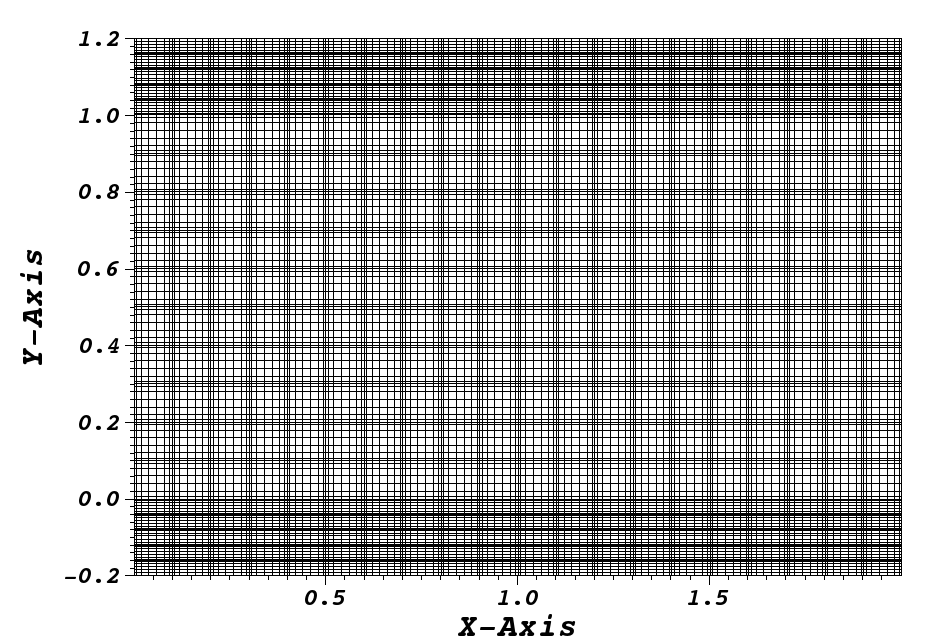
Fig. 18 Combined box mesh
usr file
The user routines file implements various subroutines to allow the users to interact with the solver.
To get started we copy the template to our case directory and then we modify its subroutines accordingly.
$ cp $HOME/Nek5000/core/zero.usr cht2d.usr
User Data
Nek5000 provides multiple subroutines useful for providing user data.
These are usrdat, usrdat2, and usrdat3 which are all called once at the begining of a run and appear towards the bottom of the template user file.
They are called at different times during initialization and the different use cases for each one can be significant, but for the purposes of this tutorial we focus only on basic input done in usrdat.
By specifying the needed user parameters in usrdat and providing them in a common block, those parameters can easily be made available to any user subroutine.
The relevant lines describing the common block are highlighted for emphasis.
Note that they will appear in most of the modified subroutines.
      subroutine usrdat()   ! This routine to modify element vertices
      implicit none
      include 'SIZE'
      include 'TOTAL'

      real deltaT,hs,lambda
      common /myparams/ deltaT,hs,lambda

      deltaT = 2.5  !temperature change across solid domain
      hs = 0.2      !thickness of solid domain
      lambda = 10.0 !ratio of solid to fluid conductivity

      return
      end
Variable properties
In the uservp subroutine, users can specifiy different variable properties for the fluid and solid subdomains independently.
As an example, the thermal diffusivity of Copper is \(\alpha = 1.1 (10 ^ {-4})\) [\(m^{2}/s\)].
The thermal diffusivity ratio of Copper and liquid metal alloy GaInSn (Pr = 0.033) is 10 and the thermal diffusivity ratio of Copper and air (Pr = 0.7) is 5.2 [Foroozani2021].
The conductivity of the solid region is set by comparing the global element number, eg, to the the total number of elements in the v-mesh, nelgv.
The highlighted line indicates where this is done:
      subroutine uservp(ix,iy,iz,eg) ! set variable properties
      implicit none
      include 'SIZE'
      include 'TOTAL'
      include 'NEKUSE'

      integer ix,iy,iz,eg,e
      real deltaT,hs,lambda
      common /myparams/ deltaT,hs,lambda

!     e = gllel(eg)

      udiff  = cpfld(ifield,1)
      utrans = cpfld(ifield,2)
      if(eg.gt.nelgv) udiff=lambda*cpfld(ifield,1)

      return
      end
Note that the properties only vary between the fluid and the solid subdomains.
Properties within the fluid and solid respectively remain constant as provided by the field coefficient array (cpfld).
Buoyancy model
To account for buoyancy, the Buossinesq approximation is used.
Rather than explicitly including a variable density, a body force of the form \(F = \rho g \beta (T-T_{ref})\) is included.
Due to the choice of non-dimensionalization, this is implemented here simply as \(F = T\).
A body force is added to Nek5000 in the userf subroutine, which is seen below.
The highlighted line indicates where the buoyancy force is added in the y-direction.
      subroutine userf(ix,iy,iz,eg) ! set acceleration term
!
!     Note: this is an acceleration term, NOT a force!
!     Thus, ffx will subsequently be multiplied by rho(x,t).
!
      implicit none
      include 'SIZE'
      include 'TOTAL'
      include 'NEKUSE'

      integer ix,iy,iz,eg,e
!     e = gllel(eg)

      ffx = 0.0
      ffy = temp
      ffz = 0.0

      return
      end
Initial & boundary conditions
The next step is to specify the initial and boundary conditions. We apply a linear variation of temperature in the fluid mesh in the y-direction where the lower surface of the lower plate is maintained at a high temperature, and the upper surface of the upper plate is maintained at a low temperature.
In this RBC example \(Ra = 10 ^ {7}\) and \(Pr= 0.033\) are choosen.
The equilibrium state of pure conductive heat transfer as the initial condition takes the form T = 1 - y for 0 < y < 1 in the fluid domain and \(T \approx 1\) and \(\approx 0\) at the fluid-solid boundaries.
It should be mentioned that the temperature drop across both solid-plates varies with Pr and Ra and it should be adjusted at the boundaries with temperature increment \(\delta T\).
One can apply a temperature increment of \(\delta T = 2.5\) at the top of the upper plate and the bottom of the lower plate for \(Pr = 0.033\) and \(\delta T = 4.72\) for \(Pr = 0.7\) as depicted in Fig. 19.
Subsequently, we modify userbc and useric as:
      subroutine userbc(ix,iy,iz,iside,eg) ! set up boundary conditions
!
!     NOTE ::: This subroutine MAY NOT be called by every process
!
      implicit none
      include 'SIZE'
      include 'TOTAL'
      include 'NEKUSE'

      integer ix,iy,iz,iside,eg
      real deltaT,hs,lambda
      common /myparams/ deltaT,hs,lambda

!      if (cbc(iside,gllel(eg),ifield).eq.'v01')

      ux   = 0.0
      uy   = 0.0
      uz   = 0.0
      temp = 0.0
      if(y.gt.1.0) temp =-deltaT !top plate
      if(y.lt.0.0) temp = deltaT !bottom plate

      return
      end
      subroutine useric(ix,iy,iz,eg) ! set up initial conditions
      implicit none
      include 'SIZE'
      include 'TOTAL'
      include 'NEKUSE'

      integer ix,iy,iz,eg
      real deltaT,hs,lambda
      common /myparams/ deltaT,hs,lambda

      ux   = 0.0
      uy   = 0.0
      uz   = 0.0
      temp = 1.0 - y !fluid temperature

      if(y.ge.1.0) then
        temp = 1.0 - ( y / hs ) * deltaT !top plate
      elseif(y.le.0.0) then
        temp = ( 1.0 - y ) / hs * deltaT !bottom plate
      endif

      return
      end
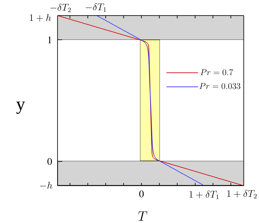
Fig. 19 Mean dimensionless temperature profiles in the CHT setting. Temprerature variation in solid-fluid domain is shown here.
Control parameters
The control parameters for any case are given in the .par file.
For this case, using any text editor, create a new file called cht2d.par and type in the following:
# Nek5000 parameter file
[GENERAL]
stopAt = endTime
endTime = 50
dt = 5.0e-1
variabledt = yes
targetCFL = 0.5
writeControl = runTime
writeInterval = 1.0

[VELOCITY]
density = 1.0
# viscosity = sqrt(1/Ra)
viscosity = 5.744563e-5

[TEMPERATURE]
conjugateHeatTransfer = yes
rhoCp = 1.0
# conductivity = sqrt(Ra * Pr)
conductivity = 1.740776e-3
Note that if the file cht2d.rea exists within the case directory, Nek5000 will preferentially read the case parameters from that file instead, which may result in errors or inconsistent results.
In this example, we have set the calculation to stop after a physical time of 50 (endTime = 50.0) and write the checkpoint file every 1 physical time units (writeInterval = 1.0).
This will provide 50 snapshots of the developing velocity and temperature fields.
In choosing viscosity = 5.744563E-05 and conductivity = 1.740776E-03, actually we are setting the Rayleigh Ra=10e7 and Pr=0.033.
By omitting the [PRESSURE] and [PROBLEMTYPE] categories, we are telling the solver to use default values for the necessary parameters.
Additional details on available settings in the par file are available here.
SIZE file
The static memory layout of Nek5000 requires the user to set some solver parameters through a so called SIZE file.
Typically it’s a good idea to start from the template.
If you haven’t already, copy the SIZE.template file from the core directory and rename it SIZE in the working directory:
$ cp $HOME/Nek5000/core/SIZE.template SIZE
Then, adjust the following parameters in the BASIC section. The only one you will likely need to change is the number of global elements on the highlighted line.
      ! BASIC
      parameter (ldim=2)               ! domain dimension (2 or 3)
      parameter (lx1=8)                ! GLL points per element along each direction
      parameter (lxd=12)               ! GL  points for over-integration (dealiasing)
      parameter (lx2=lx1-0)            ! GLL points for pressure (lx1 or lx1-2)

      parameter (lelg=400)             ! max number of global elements
      parameter (lpmin=1)              ! min number of MPI ranks
      parameter (lelt=lelg/lpmin + 3)  ! max number of local elements per MPI rank
      parameter (ldimt=1)              ! max auxiliary fields (temperature + scalars)
For this tutorial we have set our polynomial order to be \(N=7\) - this is defined in the SIZE file above as lx1=8 which indices that there are 8 points in each spatial dimension of every element.
Additional details on the parameters in the SIZE file are given here.
Compilation
You should now be all set to compile and run your case! As a final check, you should have the following files:
If for some reason you encountered an insurmountable error and were unable to generate any of the required files, you may use the provided links to download them. After confirming that you have all five, you are now ready to compile
$ makenek cht2d
If all works properly, upon compilation the executable nek5000 will be generated and you will see something like:
#############################################################
#                  Compilation successful!                  #
#############################################################
   text	   data	    bss	    dec	    hex	filename
1774311	  16940	141305600	143096851	8877c13	nek5000
Note that compilation only relies on the user file and the SIZE file. Any changes to these two files will require recompiling your case! Now you are all set, just run
$ nekbmpi cht2d 4
to launch an MPI jobs on your local machine using 4 ranks. The output will be redirected to logfile.
Post-processing the results
Once execution is completed your directory should now contain multiple checkpoint files that look like this:
cht2d.f00001
cht2d.f00002
...
The preferred mode for data visualization with Nek5000 is to use Visit or Paraview.
This requires generating a metadata file with visnek, found in /scripts.
It can be run with
$ visnek cht2d
to obtain a file named cht2d.nek5000.
This file can be opened with either Visit or Paraview.
In the viewing window, the temperature-field can be visualized. It will be similar to, but not necessarily identical to that shown in Fig. 20.
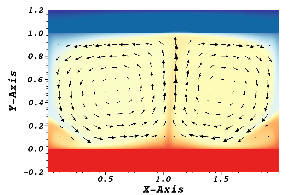
Fig. 20 Steady-State flow field visualized in Visit. Vectors represent velocity. Colors represent temperature.