RANS Channel
This tutorial describes the essential setup details for a wall-resolved RANS simulation, illustrated through a 2D channel case. The \(k-\tau\) RANS model is employed for this tutorial, which is the recommended RANS model in Nek5000. Other RANS models, including the regularized \(k-\omega\), are also available. For more information see here.
Before You Begin
It is highly recommended that new users familiarize themselves with the basic Nek5000 simulation setup files and procedures outlined in the Fully Developed Laminar Flow and Periodic Hill tutorials before proceeding.
Warning
The RANS models rely on setting an implicit source term for robustness. This is not supported in V19 or earlier versions of Nek5000. Any implementation of RANS models should use the latest master branch from github.
Mesh and Boundary Conditions
The mesh is generated with genbox using the following input file
-2                    spatial dimension
1                     number of fields (U)
#=======================================================================
#
#    Example of .box file for channel flow
#    Note that the character bcs _must_ have 3 characters.
#
#=======================================================================
#
Box
-3  -7                                nelx,nely,nelz for Box
-0.5 0.5 1.0                             x0,x1,gain
0.0 1.0 0.35
P  ,P  ,SYM,W
It creates an infinite 2D half-channel of non-dimensional width \(1\).
The streamwise (\(x\)) direction has 3 elements with periodic (P) boundary conditions.
The spanwise (\(y\)) direction has 7 geometrically spaced elements with a symmetry (SYM) boundary condition specified at the bottom face and a wall (W) boundary on the top face.
The elements shrink from the bottom of the domain to the top with a ratio of \(0.35\).
Note
Boundary conditions for the turbulent scalars are handled internally by Nek5000 in the rans_init subroutine and do not need to be specified at the time of mesh generation.
Control Parameters (.par file)
Details of the structure of the parameter file can be found here.
For RANS simulations it is critical to include two additional scalars which correspond to the \(k\) and
\(\tau\) fields respectively.
Here, they are included as the [SCALAR01] and [SCALAR02] cards.
In addition, it is essential to also include the [PROBLEMTYPE] card and enable variableProperties and stressFormulation.
For this particular tutorial, the simulation is non-dimensionalized and flow properties are density=1.0 and viscosity=-125000.
It is strongly recommended to run RANS simulations in non-dimensional form.
By assigning a negative value to the viscosity, Nek5000 will treat it as a Reynolds number.
This setup corresponds to \(Re = 125,000\), which is well above the critical Reynolds number for a channel.
density and diffusivity for SCALAR01 and SCALAR02 are not used by the solver, but should be assigned identical values as density and viscosity for velocity field for consistency.
Note
Property values for turblent scalars will be replaced with those specified for the velocity field.
#
# nek parameter file
#
[GENERAL]
numSteps = 60000
dt = 5.0e-3
writeInterval = 20000
constFlowRate = X
meanVelocity = 1.0

[PROBLEMTYPE]
variableProperties = yes
stressFormulation = yes

[MESH]
numberOfBCFields = 1

[PRESSURE]
residualTol = 1.0e-5

[VELOCITY]
density = 1.0
viscosity = -125000.0
residualTol = 1.0e-6

#tke
[SCALAR01]
density = 1.0
diffusivity = -125000.0
residualTol = 1.0e-6

#tau
[SCALAR02]
density = 1.0
diffusivity = -125000.0
residualTol = 1.0e-6
The Temperature field is not solved in this tutorial, but can be turned on by adding the [TEMPERATURE] card and the requisite properties.
User Routines (.usr file)
This section describes the essential code snippets required in the .usr file for RANS simulations.
Other details of all the subroutines can be found here.
Foremost, it is essential to include the following header at the beginning of the .usr file.
include "experimental/rans_komg.f"
Files in the above relative locations in the Nek5000 repo load the essential RANS subroutines.
RANS initialization is done through the rans_init subroutine call from usrdat2.
The required code snippet is shown below.
      implicit none
      include 'SIZE'
      include 'TOTAL'

      real wd
      common /walldist/ wd(lx1,ly1,lz1,lelv)

      common /rans_usr/ ifld_tke, ifld_tau, m_id
      integer ifld_tke,ifld_tau, m_id

      integer w_id
      real coeffs(30) !array for passing your own coeffs
      logical ifcoeffs

      ifld_tke = 3 !address of tke equation in t array
      ifld_tau = 4 !address of omega equation in t array
      ifcoeffs =.false. !set to true to pass your own coeffs

C     Supported models:
c     m_id = 0 !regularized standard k-omega (no wall functions)
c     m_id = 1 !regularized low-Re k-omega (no wall functions)
c     m_id = 2 !regularized standard k-omega SST (no wall functions)
c     m_id = 3 !Not supported
      m_id = 4 !standard k-tau
c     m_id = 5 !low Re k-tau
c     m_id = 6 !standard k-tau SST

C     Wall distance function:
c     w_id = 0 ! user specified
c     w_id = 1 ! cheap_dist (path to wall, may work better for periodic boundaries)
      w_id = 2 ! distf (coordinate difference, provides smoother function)

      call rans_init(ifld_tke,ifld_tau,ifcoeffs,coeffs,w_id,wd,m_id)

      return
      end
c-----------------------------------------------------------------------
The rans_init subroutine sets up the necessary solver variables to use RANS models.
This includes loading the model coefficients, setting up the character boundary condition (cbc) array for the turbulent scalars, and calculating the regularization [Tombo2018] for the \(k-\omega\) models.
The ifld_tke and ifld_tau variables specify the field index location of the transport variables of the two-equation RANS model.
The specific RANS model used is identified by the m_id variable.
All available RANS models are annotated in the above code.
The recommended \(k-\tau\) model is invoked with m_id=4.
Selecting ifcoeffs=.false. sets the standard RANS coefficients outlined in [Wilcox2008].
Advanced users have the option of specifying their own coefficients which have to populated in the coeffs array, with ifcoeffs=.true..
The final parameter to be aware of is the wall distance function code w_id.
The recommended value for it is w_id=2 which provides a smoother distance function, populated in the wd array.
A cheaper option is available through w_id=1 which provides “taxicab” distance and can search across periodic boundaries.
The user also has the option of specifying their own wall distance array by setting w_id=0 which will require wd array to
be populated with user computed wall distance before the rans_init call.
Diffusion coefficients for all fields in RANS simulation runs must be modified to include eddy viscosity.
This is done by the following inclusions in the uservp subroutine
      implicit none
      include 'SIZE'
      include 'TOTAL'
      include 'NEKUSE'

      integer ix,iy,iz,e,eg

      common /rans_usr/ ifld_tke, ifld_tau, m_id
      integer ifld_tke,ifld_tau, m_id

      real rans_mut,rans_mutsk,rans_mutso,rans_turbPrandtl
      real mu_t,Pr_t

      e = gllel(eg)

      Pr_t=rans_turbPrandtl()
      mu_t=rans_mut(ix,iy,iz,e)

      if(ifield.eq.1) then
        udiff  = cpfld(ifield,1)+mu_t
        utrans = cpfld(ifield,2)
      else if(ifield.eq.2) then
        udiff  = cpfld(ifield,1)+mu_t*cpfld(ifield,2)/(Pr_t*cpfld(1,2))
        utrans = cpfld(ifield,2)
      else if(ifield.eq.ifld_tke) then
        udiff  = cpfld(1,1)+rans_mutsk(ix,iy,iz,e)
        utrans = cpfld(1,2)
      else if(ifield.eq.ifld_tau) then
        udiff  = cpfld(1,1)+rans_mutso(ix,iy,iz,e)
        utrans = cpfld(1,2)
      end if

      return
      end
c-----------------------------------------------------------------------
As above, eddy viscosity, mu_t, is added to the momentum diffusion coefficient and \(k\) and \(\tau\) diffusion coefficients are modified as described by Eq. (25) in the RANS theory section.
Note
The transport and diffusion coefficients (utrans and udiff) for the RANS scalars are set with the field coefficient array vaules (cpfld) for field 1, velocity. This is done to ensure consistency in the problem setup.
Source terms in the \(k-\tau\) transport equations, Eq. (25), are added with the following inputs in the userq subroutine
      implicit none
      include 'SIZE'
      include 'TOTAL'
      include 'NEKUSE'

      common /rans_usr/ ifld_tke, ifld_tau, m_id
      integer ifld_tke,ifld_tau, m_id

      real rans_kSrc,rans_omgSrc
      real rans_kDiag,rans_omgDiag

      integer ie,ix,iy,iz,ieg
      ie = gllel(ieg)

      if (ifield.eq.2) then
        qvol = 0.0
        avol = 0.0
      else if (ifield.eq.ifld_tke) then
        qvol = rans_kSrc  (ix,iy,iz,ie)
        avol = rans_kDiag (ix,iy,iz,ie)
      else if (ifield.eq.ifld_tau) then
        qvol = rans_omgSrc (ix,iy,iz,ie)
        avol = rans_omgDiag(ix,iy,iz,ie)
      end if

      return
      end
c-----------------------------------------------------------------------
Implicit source terms contributions are specified to the avol variable, while remaining terms are
in the qvol variable.
For the wall-resolved \(k-\tau\) RANS model, the wall boundary conditions for \(k\) and \(\tau\) are both zero.
These are set in userbc as
      implicit none
      include 'SIZE'
      include 'TOTAL'
      include 'NEKUSE'
c
      integer ix,iy,iz,iside,e,eg
      character*3 cb1

      common /rans_usr/ ifld_tke, ifld_tau, m_id
      integer ifld_tke,ifld_tau, m_id

      e = gllel(eg)
      cb1 = cbc(iside,e,1) !velocity boundary condition

      ux   = 0.0
      uy   = 0.0
      uz   = 0.0
      temp = 0.0

      if(cb1.eq.'W  ') then
        if(ifield.eq.ifld_tke) then
          temp = 0.0
        else if(ifield.eq.ifld_tau) then
          temp = 0.0
        end if
      end if

      return
      end
c-----------------------------------------------------------------------
The velocity boundary condition is checked in cb1 for a wall on the highlighted line.
For this periodic case, this is not strictly necessary.
However, for any inlet/outlet case it is needed to distinguish between the Dirichlet BC values for \(k\) and \(\tau\) on the wall versus an inlet, where cb1 would have a value of v.
Initial conditions are specified in the useric routine.
For RANS simulations, positive non-zero initial values for \(k\) and \(\tau\) are recommended.
The following is used for the channel simulation,
      implicit none
      include 'SIZE'
      include 'TOTAL'
      include 'NEKUSE'

      integer ix,iy,iz,e,eg

      common /rans_usr/ ifld_tke, ifld_tau, m_id
      integer ifld_tke,ifld_tau, m_id

      e = gllel(eg)

      ux   = 1.0
      uy   = 0.0
      uz   = 0.0
      temp = 0.0

      if(ifield.eq.ifld_tke) temp = 0.01
      if(ifield.eq.ifld_tau) temp = 0.2

      return
      end
c-----------------------------------------------------------------------
SIZE file
The SIZE file can be copied from the available template included at the Nek5000/core/SIZE.template and changing the basic parameters as necessary for this case.
The user needs to ensure that the auxiliary fields specified in the SIZE file is at minimum ldimt=3 for RANS simulations.
This includes the reserved field for temperature and the two additional fields for the turbulent scalars.
In order to use the stress formulation, additional memory must be allocated by setting, lx1m=lx1
These two changes are highlighted below.
Other details on the contents of the SIZE file can be found here.
      ! BASIC
      parameter (ldim=2)               ! domain dimension (2 or 3)
      parameter (lx1=8)                ! GLL points per element along each direction
      parameter (lxd=12)               ! GL  points for over-integration (dealiasing)
      parameter (lx2=lx1)              ! GLL points for pressure (lx1 or lx1-2)

      parameter (lelg=3*7)             ! max number of global elements
      parameter (lpmin=1)              ! min number of MPI ranks
      parameter (lelt=lelg/lpmin + 3)  ! max number of local elements per MPI rank
      parameter (ldimt=3)              ! max auxiliary fields (temperature + scalars)

      ! OPTIONAL
      parameter (ldimt_proj=1)         ! max auxiliary fields residual projection
      parameter (lelr=lelt)            ! max number of local elements per restart file
      parameter (lhis=1001)            ! max history/monitoring points
      parameter (maxobj=1)             ! max number of objects
      parameter (lpert=1)              ! max number of perturbations
      parameter (toteq=1)              ! max number of conserved scalars in CMT
      parameter (nsessmax=1)           ! max sessions to NEKNEK
      parameter (lxo=lx1)              ! max GLL points on output (lxo>=lx1)
      parameter (mxprev=20)            ! max dim of projection space
      parameter (lgmres=30)            ! max dim Krylov space
      parameter (lorder=3)             ! max order in time
      parameter (lx1m=lx1)             ! GLL points mesh solver
      parameter (lfdm=0)               ! unused
      parameter (lelx=1,lely=1,lelz=1) ! global tensor mesh dimensions

      parameter (lbelt=1)              ! lelt for mhd
      parameter (lpelt=1)              ! lelt for linear stability
      parameter (lcvelt=1)             ! lelt for cvode
Compilation
All required case files for RANS wall-resolved channel simulation can be downloaded using the links below:
Results
For reference, the results obtained from the \(k-\tau\) RANS wall-resolved simulation are shown below and
compared with results from low-Re \(k-\tau\) (m_id=5), regularized \(k-\omega\) (m_id=0) and low-Re regularized
\(k-\omega\) (m_id=1) models.
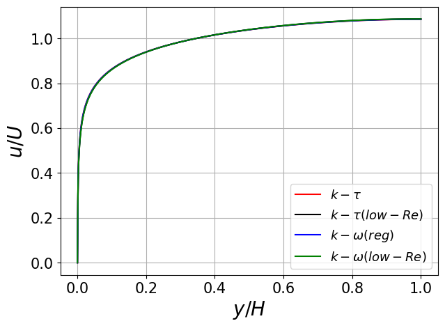
Fig. 23 Normalized stream-wise velocity from different RANS models.
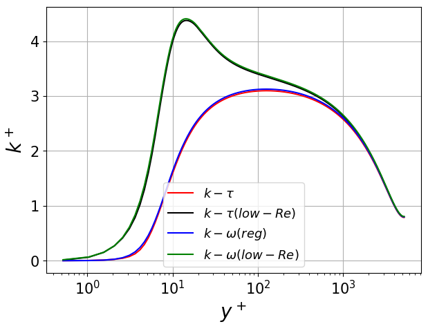
Fig. 24 Normalized TKE from different RANS models.
RANS models may be simply switched by using the appropriate m_id in usrdat2.
The low-Re versions of the model should be employed only for capturing the near wall TKE peak.
It may require additional resolution in the near-wall region and has only minimal impact on the velocity profile.