Multi-Component RANS

This is an advanced tutorial comprising RANS simulation in a multi-component geometry. The components include an inlet nozzle coupled with a wire-pin bundle. Given the scale of the geometry and mesh used in this tutorial, it is assumed that the user has access to a computing cluster for running the case. The final mesh for the inlet nozzle contains 662,360 hexahedral elements and the wire-wrapped fuel bundle contains 207,360 hexahedral elements. The NekNek module is used for interfacing between the two components, allowing for runtime transfer of field data and coupled simultaneous solution of the flow and temperature equations. The tutorial employs several advanced Nek5000 tools, procedures and user routines including

• exo2nek for importing third party mesh file to Nek5000
• reatore2 for converting ASCII Nek5000 mesh to binary format
• gencon for generating mesh connectivity file
• wiremesher for generating wire-wrapped pin bundle mesh
• nekamg_setup for generating algebraic multi-grid solver (AMG) files
• \(k-\tau\) RANS simulation setup
• NekNek setup

Before You Begin

It is highly recommended that new users familiarize themselves with the basic Nek5000 simulation setup files and procedures outlined in the Fully Developed Laminar Flow and Periodic Hill tutorials. Further, some sections of the tutorial will assume familiarity with RANS Channel and Overlapping Overset Grids tutorials.

Warning

The RANS models rely on setting an implicit source term for robustness. This is not supported in V19 or earlier versions of Nek5000. Any implementation of RANS models should use the latest master branch from github.

Case Overview

All required files for this tutorial can be downloaded using the following link:

• inlet_bundle.tar.gz

Extract the above tar file and navigate to the inlet_bundle (parent) directory

$ tar -xzvf inlet_bundle.tar.gz
$ cd inlet_bundle

It has the following directories and files, discussed in detail in the following sections:

• inletMesh –> Directory containing inlet mesh related files.
• bundleMesh –> Directory containing pin-wire bundle mesh related files.
• SIZE –> Parameter file for defining problem size.
• inlet_bundle.usr –> Fortran file for user specified subroutines.
• inlet.par –> Nek5000 parameter file.
• bundle.par –> Nek5000 parameter file.
• SPLINE –> Common block Fortran file for spline interpolation.
• InletProf.dat –> Inlet condition data file.
• neknekk –> Sample script for launching NekNek job (on Sawtooth cluster).

Geometry Description

The geometry under consideration consists of two components including an inlet nozzle connected to a wire-wrapped pin bundle. These are shown below with the inlet nozzle domain in red and the pin bundle domain in light gray. The bundle geometry is based loosely on the Advanced Burner Reactor [Grandy2007] and the inlet nozzle is based on designs considered for the Versatile Test Reactor [Yoon2021].

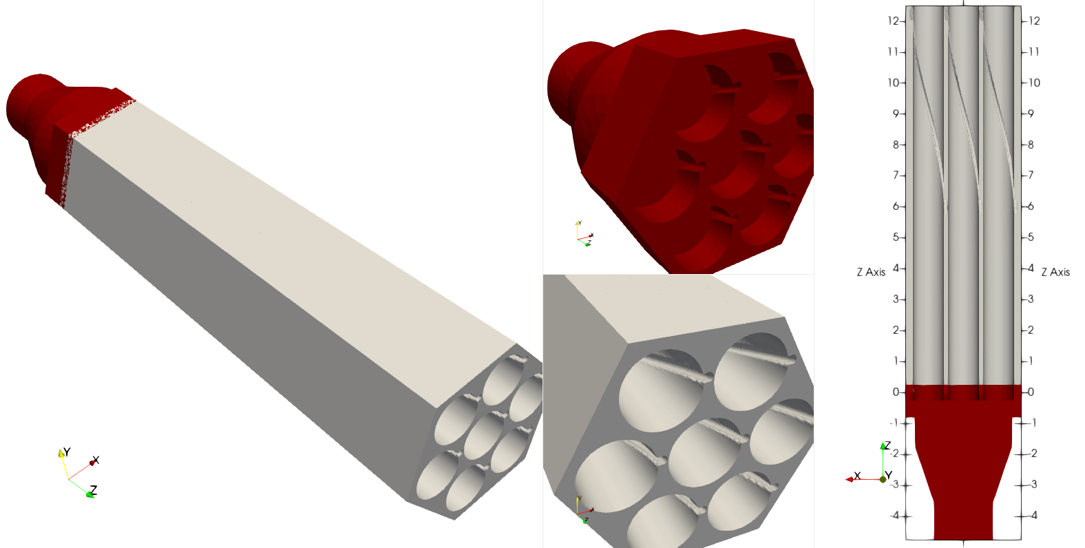
Fig. 25 Component geometries including an inlet nozzle (red) connected to a wire-wrapped pin bundle (gray)

The geometry is non-dimensionalized with respect to the pin diameter, \(D\). The axial extent of the inlet nozzle component is \(z/D=[-4.75,0.25]\) and the wire-pin bundle axial dimensions are \(z/D=[0,12.5]\). The two components, therefore, have an axial overlap of \(\Delta z/D= 0.25\), while the lateral dimensions are conformal. The inlet nozzle has an inlet diameter of \(D_{in}/D=1.875\).

Note

A reasonable overlap in the computational domains is imperative for a robust NekNek simulation. As a general rule, increasing the extent of overlap will render more stability to the coupled solver.

The Pitch-to-diameter ratio of the wire-pin bundle is 1.13 and the wire diameter is \(D_w/D=0.12875\). To prevent sharp corners, a fillet of diameter \(D_f/D=0.05\) is introduced between the pin and the wire and the wire is slightly submerged in the pin by a distance of \(0.025D_w\). The side length of the hexagonal bundle is \(1.865D\) and the diameter of the inlet nozzle boundary is \(D_{in}/D=1.875\). The length of the bundle component is equal to the wire pitch, \(L_b/D=12.5\). All geometric values are given in both dimensional and dimensionless form in the next section in Table 29 along with other flow parameters.

Thermal-hydraulic Parameters and Boundary Conditions

For non-dimensionalizing this case, the pin diameter and inlet velocity are chosen as reference values. This leads to the definition of Reynolds number as

\[Re = \frac{U_{in}D_{pin}}{\nu}\]

It is also useful to define the inlet Reynolds number as

\[Re_{in} = \frac{U_{in}D_{in}}{\nu}=\frac{D_{in}}{D_{pin}}Re\]

and an alternate bundle Reynolds number as

\[Re_b = \frac{U_{b}D_h}{\nu}=\frac{A_{in}}{A_{b}}\frac{D_h}{D_{pin}}Re\]

The bundle area is approximated as

\[A_b = A_{hex} - N_{pins}\frac{\pi}{4}\left( D_{pin}^2 + D_w^2\right)\]

and the hydraulic diameter as

\[D_h = \frac{4 A_b}{P_{hex}+N_{pins}\pi\left(D_{pin}+D_w\right)}\]

For this case, an inlet velocity of \(U_{in}=1\) m/s was chosen. This gives an inlet Reynolds number of \(Re_{in}=60,000\), a bundle Reynolds number of \(Re_b\approx9800\), and a case Reynolds number of \(Re = 32,000\) All flow and thermal properties are listed in Table 29.

A no-slip boundary condition is specified on all walls and the corresponding values of \(k\) and \(\tau\) on the walls is zero. A constant non-dimensional temperature \(T^*=1\) is specified at the inlet and a non-dimensional heat flux of \(q'' =1\) is applied on the pin walls from half axial length of the bundle. An insulated wall condition is specified on all remaining boundaries. A Prandtl number of 0.005 was chosen corresponding to liquid Sodium and an increased turbulent Prandtl number was chosen to account for turbulent mixing.

Table 29 Flow and Thermal Properties

Parameter	Variable	Dimensional Value	Dimensionless Value
Pin diameter	\(D_{pin}\)	\(8\) mm	\(1\) (reference)
Wire diameter	\(D_{w}\)	\(1.03\) mm	\(0.129\)
Inlet diameter	\(D_{in}\)	\(15\) mm	\(1.875\)
Hydraulic diameter	\(D_h\)	\(3.06\) mm	\(0.383\)
Inlet velocity	\(U_{in}\)	\(1.0\) m/s	\(1\) (reference)
Bundle velocity	\(U_b\)	\(0.801\) m/s	\(0.801\)
Kinematic viscosity	\(\nu\)	\(2.5\cdot(10^{-7})\) m2/s	\(3.125\cdot(10^{-5})\)
Thermal diffusivity	\(\alpha\)	\(5.0\cdot(10^{-5})\) m2/s	\(6.25\cdot(10^{-3})\)
Reynolds number	\(Re\)	–	\(32000\)
Inlet Reynolds number	\(Re_{in}\)	–	\(60000\)
Bundle Reynolds number	\(Re_{b}\)	–	\(9814\)
Prandtl number	\(Pr\)	–	\(0.005\)
Peclet number	\(Pe\)	–	\(160\)
Turbulent Prandtl number	\(Pr_t\)	–	\(1.5\)

Mesh Generation

Inlet Nozzle (exo2nek)

A third-party meshing tool (e.g., ANSYS ICEM) is required for generating the mesh for the inlet component. In this case, the mesh was saved as an EXODUS II (.exo) mesh file. Nek5000 offers the exo2nek mesh conversion tool for converting an .exo mesh file to .re2 format, as well as gmsh2nek for converting .msh files from Gmsh. For more information see exo2nek.

By default, all Nektools support only 150,000 elements. To run this case, exo2nek and gencon will need to be compiled with support for considerably more elements. To do this, go to the Nek5000/tools directory and edit the maketools file.

$ cd ~/Nek5000/tools
$ vi maketools

Uncomment the line specifying the maximum number of elements and change it to a value larger than the number of elements in the largest mesh, such as that shown on the highlighted line below.

#!/bin/bash

# maximum number of elements
MAXNEL=1000000

# binary path
#bin_nek_tools=`cd ../bin && pwd`

# Fortran compiler
#FC="gfortran"
#FFLAGS=""

# C compiler
#CC="gcc"
#CFLAGS=""

# linking flags
#LDFLAGS="-L$HOME/lib -lm"

source ./maketools.inc

The exo2nek and gencon tools can then be recompiled with

$ ./maketools exo2nek gencon

Note

If you still get errors about the tools not supporting enough elements, you may need to delete the exo2nek or gencon binary in Nek5000/bin and the corresponding *.o files in the tool’s subdirectory manually before recompiling. Executing $ ./maketools clean will also work, but this will delete all of the tools.

The above command will compile the exo2nek and gencon tools. The latter is required for generating the mesh connectivity file at a later step.

Currently, exo2nek supports the following mesh elements,

• 1^st order tetrahedra, TET4
• 1^st order wedges, WEDGE6
• 1^st order hexahedra, HEX8
• 2^nd order tetrahedra, TET10
• 2^nd order wedges, WEDGE15
• 2^nd order hexahedra, HEX20

The user must ensure that the third-party mesh comprises only the above listed element types. The inlet.exo file included with this tutorial contains 165590 TET4 elements. The exo2nek tool includes built-in tet-to-hex and wedge-to-hex conversions, so the 165590 tetrahedral elements will be converted to 662360 hexahedral elements. Navigate to the folder containing inlet mesh and run exo2nek.

$ cd inletMesh
$ exo2nek

The output from exo2nek is shown below, where the expected user input is highlighted. The inputs are explained as:

• We are converting the file inlet.exo, where the .exo file extension is implied.
• This case does not use a conjugate heat transfer model, so there are 0 solid .exo files.
• This case is not periodic, so there are 0 periodic boundary surface pairs.
• The produced file will be named inlet.re2, where the .re2 file extension is again implied.

 please input number of fluid exo files:
1
 please input exo file:
inlet

inlet.exo                        is an EXODUSII file; version 0.00
I/O word size 8

database parameters:

title         =  Created by ICEMCFD - EXODUS II Interface

num_dim       =        3
num_nodes     =    35901
num_elem      =   165590
num_elem_blk  =        1
num_side_sets =        3

element block id   =        1
element type       =    TETRA
num_elem_in_block  =   165590
num_nodes_per_elem =        4

 TETRA4 is valid element in a 3D mesh.
 assume linear hybrid mesh (tetra-hex-wedge)
 one TETRA4 divide into 4 Nek hex elements
 please input number of solid exo files for CHT problem (input 0 for no solid mesh):
0
 done pre-read exo files
 now converting to nek mesh


Store SideSet information from EXO file
Sideset  2 ...
Sideset  3 ...
Sideset  4 ...

Converting elements ...
 flag1
 flag2
 Converting elements in block            1
 nvert,                     4
 Converted elements in nek:               662360
Done :: Converting elements
 Domain max xyz:   1.8650400000000000        1.6151700000000000       0.25000000000000000
 Domain min xyz:  -1.8650400000000000       -1.6151700000000002       -4.7500000000000000
 total element now is                662360
 fluid exo file            1  has elements       662360
 calling: gather_bc_info()
 done: gather_bc_info()
 ******************************************************
 Boundary info summary
 sideSet ID
           2
           3
           4
 ******************************************************
 Enter number of periodic boundary surface pairs:
0
 please give re2 file name:
inlet

writing inlet.re2
 velocity boundary faces:        95148

Following the above steps will generate the file inlet.re2 in the current directory. For the inlet nozzle component, the following boundary IDs are assigned:

• 2 –> Nozzle inlet
• 3 –> Interfacing surface (nozzle outlet/bundle inlet)
• 4 –> Walls

These are generated from the sideset numbers assigned when generating the original mesh. As a basic sanity check, exo2nek prints out any sideset IDs it finds.

Note

The sideSet ID for all mesh boundaries must be specified in the .exo file using the third-party meshing software of the user’s choice. These values are accessible in Nek5000 in the BoundaryID array.

Return and move the mesh file to the parent directory:

$ cd ../
$ mv inletMesh/inlet.re2 .

Wire-pin Bundle (wiremesher)

To generate the pin-wire bundle mesh, navigate to the wireMesh folder:

$ cd wireMesh

It contains two sub-directories, viz., wire2nek and matlab. Input parameters for the meshing script are specified in the header of the matlab/wire_mesher.m file, as shown:

% Mesh parameters %%%%%%%%%%%%%%%%%%%%%%%%%%%%%%%%%%%%%%%%%%%%%%%%%%%%%%%%%
D    = 8.00;            %  pin diameter  (mm)
P    = 9.04;            %  pin pitch
Dw   = 1.03;            %  wire diameter (mm)
Df   = 0.4;             %  fillet diameter (mm) (making this too small can cause bad elements)
H    = 100.0;           %  wire pitch (mm)
T    = 0.05*Dw          % trimmed off of wire (mm) (cuts off the tip of the wire)
S    = 0.025*Dw;        % Wire submerged (mm) (how sunken in the wire is into the pin)
Adjust = 1;             % if 1, Adjust flattness of wire when away from pins (if trimmed is on, only trim when wire passes pin)
iFtF   = 0;             % if 1, add layer next to outer can
G  = 0.0525;            % gap between wire and wall (mm)
FtF_rescale = 1.0086;   % rescaling of outer FtF, the difference is given by an additional mesh layer - MUST BE BIGGER THAN 1
ne=2;                   % Number of edge pins. e.g., ne=3 for 19 pin assembly. MINIMUM is 2
Col=12;                 % Number of columns per block (5 or 6 blocks surround each pin)
Row=3;                  % Number of rows per block (2 blocks fit between neighboring pins)
Rowdist=[65 30 5];      % distribution of elements in the row (for creating boundary layer)
Lay=20;                 % Number of layers for 60 degree turn (this should be a reasonable number - above 10, tested typically for ~20)
rperiodic=1.0;          % Less than zero if periodic, Greater than zero if inlet/outlet
ipolar=0.25*(D/H)*360   % Starting polar orientation of wire (in degrees)
%%%%%%%%%%%%%%%%%%%%%%%%%%%%%%%%%%%%%%%%%%%%%%%%%%%%%%%%%%%%%%%%%%%%%%%%%%%

All input variables are annotated in the above code snippet. Although all input dimensions shown are in mm, the script produces the wiremesh in non-dimensional units, normalized with pin diameter D. It will usually take some heuristic experimentation to specify optimum parameters based on user requirements (such as resolution, number of elements, etc.). Additionally some combinations of parameters may result in invalid elements with small or negative Jacobians. Critical parameters, that control the mesh resolution and contribute towards a successful mesh, include:

• Df –> Higher fillet diameter will be less likely to cause any errors and produce a smoother mesh. Should be adjusted to a reasonable value.
• T –> Trims off a portion of the wire to avoid pinching between the wire and neighboring pin. Typically set to 0.05*Dw.
• S –> Submerges the wire slightly into the pin to avoid sharp corners. Typically set to \(0.025*Dw\).
• Adjust –> Ensures trimming only occurs if wire passes neighboring pins. Typically set to 1.
• iFtF –> (Deprecated) Adds a layer next to outer wall. Set to 0.
• FtF_rescale –> (Deprecated) Inactive i:math:f iFtF=0.
• G –> Controls gap between peripheral wire and outer wall. Adjust to needed value.
• ne –> controls the number of pins in the radial direction. ne=2 will produce a bundle with 7 pins, ne=3 will produce 19 pins, and so on.
• Col –> Controls the resolution in the azimuthal direction.
• Row –> Controls the resolution in radial direction.
• Rowdist –> Controls layer width distribution percentage in radial direction, from interior to pin wall. Must add up to 100 and entries must be equal to Row.
• Lay –> Controls resolution in axial direction. Specifies number of elements in axial length equal to 60 degree rotation of wire.

Note

If you encounter Jacobian errors with your mesh, try increasing the fillet diameter, Df or number of columns, Col.

The preset values included with the tarball should not be changed for this tutorial as the overlapping geometry between the components is fixed. The mesher is initiated by simply running the doall.sh bash script. Ensure that both Matlab and Python with numpy (tested with Python 3.8) are active before launching the script and that either gfortran or ifort is available. By default the wire2nek converter utility looks for gfortran. To use ifort instead, the compiler script bundleMesh/wire2nek/compile_wire2nek must be modified.

$ ./doall.sh

The script can take a while to complete. Upon completion it generates the wire_out.rea mesh file, which is a legacy ASCII mesh file for Nek5000. Convert this into the binary format by running the reatore2 tool. Follow the prompts:

Input .rea name:
wire_out

Input .rea/.re2 output name:
bundle

We finally obtain the bundle.re2 file which contains the pin-wire bundle mesh in the Nek5000 format. Boundary IDs are assigned by the wiremesher as:

• 1 –> Fuel pin, wire, and fillet walls
• 2 –> Bundle hexagonal (outer) walls
• 3 –> Axial inlet surface
• 4 –> Axial outlet surface

which are available in the .usr file in the BoundaryID array. Return and move the mesh file to the parent directory:

$ cd ../
$ mv bundleMesh/bundle.re2 .

Generating Connectivity file (.co2)

After generating the mesh files for both components, it is necessary to generate the corresponding connectivity files using the gencon tool. Note that using gencon instead of genmap – which generates map (.ma2) files – is the recommended procedure for large meshes.

Note

If compiled to support a large number of elements, genmap can be used to generate the .ma2 file as an alternative to gencon and parRSB. However, for large meshes this can take a very long time.

Users must include PARRSB in the PPLIST in the makenek file, which instructs Nek5000 to partition the mesh at run-time and requires the .co2 file instead of the .ma2 file for running the case. See Preprocessor List for details on PPLIST and makenek. It is recommended to copy makenek from Nek5000/bin into the project directory to edit.

Warning

Editing the copy of makenek in the Nek5000/bin directory directly can have unintended side-effects when trying to recompile other cases.

Run gencon from the parent folder for each mesh file. Users will be prompted to specify the mesh file name and tolerance. Use 0.01 for inlet and 0.2 (default) for the bundle mesh:

 Input .rea / .re2 name:
inlet
 reading inlet.re2
 Input mesh tolerance (default 0.2):
0.01

 Input .rea / .re2 name:
bundle
 reading bundle.re2
 Input mesh tolerance (default 0.2):
0.2

The above will generate the inlet.co2 and bundle.co2 connectivity files, respectively.

Parameter File (.par)

Using NekNek requires separate .par files for each of the components. The files are included in the parent folder and shown below:

#
#nek parameter file - inlet.par
#
[GENERAL]
#startFrom = inlet.fld
stopAt = numSteps
numSteps = 10000
dt = 1.0e-6
writeInterval = 1000
#extrapolation = OIFS
#targetCFL = 3.5

[PROBLEMTYPE]
variableProperties = yes
stressFormulation = yes

[PRESSURE]
preconditioner = semg_amg_hypre
residualTol = 1.0e-5
residualProj = yes

[VELOCITY]
density = 1.0
viscosity = -32000.0
residualTol = 1.0e-6

[TEMPERATURE]
rhoCp = 1.0
conductivity = -160.0
residualTol = 1.0e-6

#tke
[SCALAR01]
density = 1.0
diffusivity = -32000.0
residualTol = 1.0e-6

#tau
[SCALAR02]
density = 1.0
diffusivity = -32000.0
residualTol = 1.0e-6

#
#nek parameter file - bundle.par
#
[GENERAL]
#startFrom = bundle.fld
stopAt = numSteps
numSteps = 10000
dt = 1.0e-6
writeInterval = 1000
#extrapolation = OIFS
#targeCFL = 3.5
 
[PROBLEMTYPE]
variableProperties = yes
stressFormulation = yes

[PRESSURE]
preconditioner = semg_amg_hypre
residualTol = 1.0e-5
residualProj = yes

[VELOCITY]
density = 1.0
viscosity = -32000.0
residualTol = 1.0e-6

[TEMPERATURE]
rhoCp = 1.0
conductivity = -160.0
residualTol = 1.0e-6

#tke
[SCALAR01]
density = 1.0
diffusivity = -32000.0
residualTol = 1.0e-6

#tau
[SCALAR02]
density = 1.0
diffusivity = -32000.0
residualTol = 1.0e-6

Both parameter files are identical, except for one important difference. To restart the case from any given time, separate restart file names should be specified to the startFrom parameter. It is critical that the properties and time step size are identical for both .par files. Values are assigned in dimensionless form – density is set to unity, viscosity and diffusivity are set to \(-Re\) and conductivity to \(-Pe\). The negative values indicate that the solver is run in dimensionless form.

Note that given the large size of the meshes, the preconditioner must be set to semg_amg_hypre. This invokes the algebraic multigrid (AMG) solver for pressure instead of the default XXT solver. The AMG preconditioner requires third party HYPRE libraries which must be included in the preprocessor list option in the makenek file.

Note

By default, Nek5000 does not support using the default XXT preconditioner for meshes with \(E\ge250,000\). Generally, the AMG preconditioners perform better for larger meshes.

As mentioned above, it is recommended to copy makenek from Nek5000/bin into the project directory to edit. Also including the PARRSB option, as mentioned earlier, the PPLIST should be:

PPLIST = "HYPRE PARRSB"

Further details on all parameters of .par file can be found here and further information on PPLIST is available here.

User Routines (.usr file)

Basics of the required setup routines for a NekNek simulation can be found in the Overlapping Overset Grids turorial, while for a RANS simulation in the RANS Channel tutorial. Although this section decribes all user routines required for a NekNek RANS simulation in detail, a comprehensive understanding of routines from these simpler cases is recommended before proceeding.

The following files are required to be included in the .usr file for loading RANS related subroutines They can be included anywhere in the .usr file outside of a subroutine, but we recommend keeping them at the top for consistency and quick reference.

      include "experimental/rans_komg.f"
      include "experimental/rans_wallfunctions.f"

NekNek related parameters are specified in usrdat routine:

      subroutine usrdat()
      include 'SIZE'
      include 'TOTAL'
      include 'NEKNEK'
      
!     ngeom - parameter controlling the number of iterations,
!     set to ngeom=2 by default (no iterations)
!     One could change the number of iterations as
      ngeom = 2
      
!     ninter - parameter controlling the order of interface extrapolation for neknek,
!     set to ninter=1 by default
!     Caution: if ninter greater than 1 is chosen, ngeom greater than 2
!     should be used for stability
      ninter = 1
      
      nfld_neknek=7             !velocity+pressure+t+sc1+sc2
      
      return
      end

The ngeom variable specifies the number of overlapping Schwarz-like iterations, while ninter controls the time extrapolation order of boundary conditions at the overlapping interface. Using ninter=1 is unconditionally stable, while a higher temporal order will typically require more iterations for stability (ngeom>2). For computational savings, we maintain first order temporal extrapolation for this tutorial. The number of total field arrays that are transferred between the two meshes is specified by nfld_neknek. For 3D RANS cases it must be equal to 7 (3 velocity, 1 pressure and 3 scalar field arrays - temperature, \(k\) and \(\tau\)).

Note

Ensure that proper common block headers are included in subroutines. The NEKNEK header is required for routines where idsess, nfld_neknek, the valint array, and other NEKNEK variables need to be accessed.

Boundary Condition specification and RANS initialization is performed in usrdat2:

c---------------------------------------------------------------------
      subroutine usrdat2()
      implicit none
      include 'SIZE'
      include 'TOTAL'
      include 'NEKNEK'
      
      real wd
      common /walldist/ wd(lx1,ly1,lz1,lelv)

      common /rans_usr/ ifld_tke, ifld_tau, m_id
      integer ifld_tke,ifld_tau, m_id
      
      integer w_id,imid,i
      real coeffs(30)           !array for passing your own coeffs
      logical ifcoeffs
      
      integer ifc,iel,id_face
      
      if(idsess.eq.0)then       !BCs for inlet mesh
         do iel=1,nelt
            do ifc=1,2*ndim
               id_face = BoundaryID(ifc,iel)
               if (id_face.eq.2) then !inlet
                  cbc(ifc,iel,1) = 'v  '
                  cbc(ifc,iel,2) = 't  '
               elseif (id_face.eq.3) then !interface
                  cbc(ifc,iel,1) = 'int'
                  cbc(ifc,iel,2) = 'int'
               elseif (id_face.eq.4) then !walls
                  cbc(ifc,iel,1) = 'W  '
                  cbc(ifc,iel,2) = 'I  '
               endif
            enddo
         enddo
      else                      !BCs for pin-wire bundle mesh
         do iel=1,nelt
            do ifc=1,2*ndim
               id_face = BoundaryID(ifc,iel)
               if (id_face.eq.3) then !interface
                  cbc(ifc,iel,1) = 'int'
                  cbc(ifc,iel,2) = 'int'
               elseif (id_face.eq.4) then !outlet
                  cbc(ifc,iel,1) = 'O  '
                  cbc(ifc,iel,2) = 'O  '
               elseif (id_face.eq.1) then !pin walls
                  cbc(ifc,iel,1) = 'W  '
                  cbc(ifc,iel,2) = 'f  '
               elseif (id_face.eq.2) then !outer walls
                  cbc(ifc,iel,1) = 'W  '
                  cbc(ifc,iel,2) = 'I  '
               endif
            enddo
         enddo
      endif
      
!     RANS initialization
      ifld_tke = 3
      ifld_tau = 4
      ifcoeffs=.false.
      
      m_id = 4       ! non-regularized standard k-tau
      w_id = 2       ! distf (coordinate difference, provides smoother function)

      call rans_init(ifld_tke,ifld_tau,ifcoeffs,coeffs,w_id,wd,m_id)

      return
      end
c---------------------------------------------------------------------

The NekNek solver launches two Nek5000 sessions simultaneously and field data transfer is performed between the two sessions on each time iteration. Each session is assigned a unique sequential ID, stored in the variable idsess. Here, idsess=0 is assigned to the inlet component solve and idsess=1 to bundle component. Boundary conditions are assigned using this variable for each component, as shown above.

Note

The idsess variable is determined by the call order during job submission. See Compilation and Running for more information.

Recall the boundary IDs assigned to each component during the mesh generation process, described in the preceding section. Character codes for different boundary conditions are stored in the cbc array. Their detailed description can be found in Boundary Conditions. For each component, the nested loops go through all elements and their faces, populating cbc array for all fields based on mesh assigned boundary IDs. Note that int boundary condition must be assigned to the overlapping surfaces of the inlet and bundle components. int condition is replaced internally with Dirichlet boundary conditions subsequently by Nek5000. Flux boundary condition, f, is assigned to pin walls for temperature field while insulated, I, is assigned to all other walls.

With regards to RANS initialization; m_id=4 selects the \(k-\tau\) RANS model and w_id=2 selects the wall distance computing algorithm. \(k\) and \(\tau\) fields are stored in the 3rd and 4th index, respectively, specified with ifld_k and ifld_omega. Set ifcoeffs to .true. only if user specified RANS coefficients are required. For details on the RANS related parameters, refer RANS Channel tutorial.

Note

rans_init must be called after populating cbc array

For RANS simulation, diffusion coefficients are assigned in the uservp routine. The routine used here remains nearly identical to the RANS Channel tutorial:

      subroutine uservp (ix,iy,iz,eg)
      implicit none
      include 'SIZE'
      include 'TOTAL'
      include 'NEKUSE'
      
      integer ix,iy,iz,e,eg
      
      common /rans_usr/ ifld_tke, ifld_tau, m_id
      integer ifld_tke,ifld_tau, m_id

      real rans_mut,rans_mutsk,rans_mutso,rans_turbPrandtl
      real mu_t,Pr_t
      
      e = gllel(eg)
      
      Pr_t=1.5                  !rans_turbPrandtl()
      mu_t=rans_mut(ix,iy,iz,e)
      
      if(ifield.eq.1) then
         udiff  = cpfld(ifield,1)+mu_t
         utrans = cpfld(ifield,2)
      elseif(ifield.eq.2) then
         udiff  = cpfld(ifield,1)+mu_t*cpfld(ifield,2)/(Pr_t*cpfld(1,2))
         utrans = cpfld(ifield,2)
      elseif(ifield.eq.ifld_tke) then
         udiff  = cpfld(1,1)+rans_mutsk(ix,iy,iz,e)
         utrans = cpfld(1,2)
      elseif(ifield.eq.ifld_tau) then
         udiff  = cpfld(1,1)+rans_mutso(ix,iy,iz,e)
         utrans = cpfld(1,2)
      endif
      
      return
      end

Only turbulent Prandtl number is changed to Pr_t=1.5 for this tutorial. This value is more appropriate for molten sodium salts as compared to the default value of 0.85 (for air), which is assigned through rans_turbPrandtl() function call.

Source terms for the temperature and scalar equations are assigned through userq. The routine here is identical to the basic RANS Channel case:

      subroutine userq  (ix,iy,iz,ieg)
      implicit none
      include 'SIZE'
      include 'TOTAL'
      include 'NEKUSE'
      
      common /rans_usr/ ifld_tke, ifld_tau, m_id
      integer ifld_tke,ifld_tau, m_id
      
      real rans_kSrc,rans_omgSrc
      real rans_kDiag,rans_omgDiag
      
      integer ie,ix,iy,iz,ieg
      ie = gllel(ieg)
      
      if(ifield.eq.2) then
         qvol = 0.0
         avol = 0.0
      elseif(ifield.eq.ifld_tke) then
         qvol = rans_kSrc  (ix,iy,iz,ie)
         avol = rans_kDiag (ix,iy,iz,ie)
      elseif(ifield.eq.ifld_tau) then
         qvol = rans_omgSrc (ix,iy,iz,ie)
         avol = rans_omgDiag(ix,iy,iz,ie)
      endif
      
      return
      end

Note that either component does not have any volumetric source heat source and hence qvol=0 for temperature field (ifield.eq.2).

Initial conditions are specified in useric. Similar values are assigned to both components and, thus, the routine implementation is straightforward. Temperature is initalized to 1 for both components.

      subroutine useric (ix,iy,iz,eg)
      implicit none
      include 'SIZE'
      include 'TOTAL'
      include 'NEKUSE'
      
      integer ix,iy,iz,e,eg

      common /rans_usr/ ifld_tke, ifld_tau, m_id
      integer ifld_tke,ifld_tau, m_id
      
      e = gllel(eg)
      
      ux   = 0.0
      uy   = 0.0
      uz   = 1.0
      temp = 1.0
      
      if(ifield.eq.2) temp = 1.0
      if(ifield.eq.ifld_tke) temp = 0.01
      if(ifield.eq.ifld_tau) temp = 0.2
      
      return
      end

Boundary conditions are assigned in userbc. For the inlet component, inlet conditions are assigned using data generated from RANS simulation in a pipe with identical diameter as the inlet surface. The data is stored in the InletProf.dat file which contains axial velocity, \(k\) and \(\tau\) information as a function of radial wall distance. Two plugin subroutines are required, which perform spline interpolation of the data to the inlet mesh, viz., getInletProf and init_prof. These are provided for the user in the inlet_bundle.usr file and can be used without modification. The usage is shown below:

      subroutine userbc (ix,iy,iz,iside,eg)
      implicit none
      include 'SIZE'
      include 'TOTAL'
      include 'NEKUSE'
      include 'NEKNEK'
      
      integer ix,iy,iz,iside,eg,e

      real wd
      common /walldist/ wd(lx1,ly1,lz1,lelv)

      common /rans_usr/ ifld_tke, ifld_tau, m_id
      integer ifld_tke,ifld_tau, m_id
      
      real uin,kin,tauin,wdist
      real din,zmid

      integer id_face
      
      integer icalld
      save icalld
      data icalld /0/

      e = gllel(eg)
      
      if(icalld.eq.0)then
         call getInletProf      !Initialize spline routine
         icalld = 1
      endif
      
      ux = 0.0
      uy = 0.0
      uz = 0.0
      temp = 0.0
      flux = 0.0
      
      id_face = BoundaryID(iside,e)

      if(imask(ix,iy,iz,e).eq.0)then
         continue
      else
         ux = valint(ix,iy,iz,e,1)
         uy = valint(ix,iy,iz,e,2)
         uz = valint(ix,iy,iz,e,3)
         if(nfld_neknek.gt.3)temp = valint(ix,iy,iz,e,ldim+ifield)
      endif
      
!     Inlet condition
      if(idsess.eq.0 .and. id_face.eq.2)then
         din = 1.875            !Inlet diameter
         wdist = min(wd(ix,iy,iz,e),din/2.) !Wall distance
         call init_prof(wdist,uin,kin,tauin) !Spline interpolation from InletProf.dat
         uz = uin
         if(ifield.eq.2)temp = 1.0
         if(ifield.eq.ifld_tke)temp = kin
         if(ifield.eq.ifld_tau)temp = tauin
      endif
      
!     Heat flux on walls
      if(ifield.eq.2)then
         if(idsess.eq.0)then
            flux = 0.0
         else
            zmid = 12.5/2.0
            flux=0.0
            if(id_face.eq.1)then !Pin walls
               flux = 0.5*(1.0+tanh(2.0*PI*(zm1(ix,iy,iz,e)-zmid)))
            endif
         endif
      endif
      
      return
      end

Note that the diameter of the inlet surface is din=1.875. Spline interpolation routine, init_prof, requires the wall distance array, wd, which is populated in usrdat2 (in rans_init call). The distance should be limited to inlet radius to avoid spline from extrapolating. Inlet component is identified with idsess.eq.0 and inlet surface with its boundary ID, id_face.eq.2.

Temperature flux must also be assigned in userbc on the pin surface walls. As mentioned earlier, non-dimensional unit heat flux is assigned from half axial length of the bundle (zmid). A smoothed axial flux profile is imposed using tanh step function as shown. Flux on all remaining walls is zero.

Field data transfer between NekNek sessions is performed using valint array and the grid point locations of of overlapping boundaries are identified using the imask array. Thus, Dirichlet boundary condition values stored in valint, which contains spectral interpolation field values from overlapping mesh, are imposed at the boundary of current mesh, where imask = 1.

SIZE file

The SIZE file used for this tutorial is included in the provided tar file. The user needs to ensure that the auxiliary fields specified in the SIZE file is at minimum ldimt=3 for RANS. Further, nsessmax must be set to 2 for NEKNEK simulation. Other details on the contents of the SIZE file can be found here.

Note

The choice of lelg, lpmin, and lelt is different for a NekNek case. See the Overlapping Overset Grids tutorial for guidance.

Compilation and Running

Compile from the parent directory with the command $ ./makenek.

Warning

The makenek file was copied from Nek5000/bin and edited specifically for this case. It is imperative to include ./ in front of makenek to ensure the terminal environment executes the local version of makenek instead of the version in Nek5000/bin.

A sample script for running the case on a cluster computing environment is included in the tar file (neknekk). This script is specific to the PBS job scheduler on the Sawtooth cluster at Idaho National Laboratory. It is offered only as an example. Work with your local system administrator to develop a script to run on the cluster you have access to.

#!/usr/bin/env bash
if [[ $# -lt 6 ]] || [[ $# -gt 7 ]]; then
  echo "submission script for NekNek jobs"
  echo "usage: \$ neknekk \"session 1\" \"session 2\" \"nodes for session 1\" \"nodes for session 2\" \"hours\" \"minutes\" \"(optional) ntasks-per-node\""
  exit
fi

prj=neams

ntpn=48
[[ ! -z $7 ]] && ntpn=$7

sess1=$1
sess2=$2

nn1=$3
nn2=$4
nnt=$(($nn1 + $nn2))
np1=$(($nn1 * $ntpn))
np2=$(($nn2 * $ntpn))

ndss="nodes"
[ $nnt -eq 1 ] && ndss="node"

hrs=`printf "%02u" $5`
mns=`printf "%02u" $6`

echo "submitting NekNek job on $nnt $ndss ($ntpn ranks per node) for $hrs:$mns"

echo "     session \"$sess1\" on $np1 ranks, session \"$sess2\" on $np2 ranks"
echo "#!/bin/bash"                                    >  "neknek.batch"
echo "#PBS -N neknek"                                 >> "neknek.batch"
echo "#PBS -l select=$nnt:ncpus=$ntpn:mpiprocs=$ntpn" >> "neknek.batch"
echo "#PBS -l walltime=$hrs:$mns:00"                  >> "neknek.batch"
echo "#PBS -j oe"                                     >> "neknek.batch"
echo "#PBS -P $prj"                                   >> "neknek.batch"
echo "#PBS -o $1.out"                                 >> "neknek.batch"
echo "cd \$PBS_O_WORKDIR"                             >> "neknek.batch"
echo "export OMP_NUM_THREADS=1"                       >> "neknek.batch"
echo "echo 2 > SESSION.NAME"                          >> "neknek.batch"
echo "echo T >> SESSION.NAME"                         >> "neknek.batch"
echo "echo " $sess1 " >> SESSION.NAME"                >> "neknek.batch"
echo "echo \`pwd\`'/' >> SESSION.NAME"                >> "neknek.batch"
echo "echo " $np1 " >> SESSION.NAME"                  >> "neknek.batch"
echo "echo " $sess2 " >> SESSION.NAME"                >> "neknek.batch"
echo "echo \`pwd\`'/' >> SESSION.NAME"                >> "neknek.batch"
echo "echo " $np2 " >> SESSION.NAME"                  >> "neknek.batch"
echo rm -f  *.sch                                     >> "neknek.batch"
echo rm -f ioinfo                                     >> "neknek.batch"
echo "module purge"                                   >> "neknek.batch"
echo "module load openmpi/4.0.5_ucx1.9_gcc4.9.4"      >> "neknek.batch"
echo "mpirun ./nek5000 > logfile"                     >> "neknek.batch"
qsub neknek.batch
sleep 3
qstat -u `whoami`

This script expects at least six arguments with an optional seventh. The arguments are:

• session 1 name (must match one set of par, re2, and con files)
• session 2 name (must match the other set of input files)
• number of nodes for session 1
• number of nodes for session 2
• runtime hours
• runtime minutes (between 0 - 60)
• number of MPI ranks per node (optional, defaults to 48)

Note

The first session name given as an argument will be assigned idsess=0, with the second will be assigned idsess=1. Keep in mind how these were used in the .usr file.

As an example, the script can be launched as follows:

$ ./neknekk inlet bundle 30 10 4 30

This submits a NEKNEK job on 40 nodes (30 dedicated to the inlet nozzle and 10 dedicated to the wire-wrapped bundle) for 4 hours and 30 minutes. The combined case will likely require significantly longer runtime. As the case runs, output from both sessions will be written to a common logfile. This can make interpreting the logfile quite difficult.

Note

When running any NekNek case, the number of nodes for each session should be proportional to the number of elements.

Helpful Tips

The following tips may be helpful to make the simulations more tractable:

• Start with a small time step size and high viscosity value (low Re) to stabilize the pressure solver during initial transients.
• Accelerate the simulation by running a standalone case for the inlet component, allowing flow to evolve before using the NEKNEK solver for the coupled simulation. Replace the int boundary condition with O (outlet) for the inlet component.
• Once the case is stable, use characteristics to run the simulation at larger time steps (CFL>1). This requires the following entries in the .par file (uncomment to use):

#extrapolation = OIFS
#targetCFL = 3.5

It is necessary to specify a target CFL to use characteristics, also known as operator-integrator factor splitting. It uses a Runge-Kutta substepping method to exceed the CFL constraint. The number of substeps is based on the targetCFL value.

Warning

The characteristics require time to compute. It is not unusual for the wall-time per time step to increase by a factor of 3 or 4. It should only be used if your case can achieve at least a comparable increase in time step size. This should be tested on a case-by-case basis!

Results

Once the case has been running, it will produce output files for each session independently. They can be visualized using either ParaView or VisIt. The metadata files necessary to do this can be generated by using the visnek script.

For reference, normalized velocity magnitude and turbulent kinetic energy (TKE) contour plots are shown below along lateral cross-sections of the inlet and wire-pin bundle components. Note that the overlap plane is located at \(z=0\) axial location, where the polar orientation of wire is \(7.2^{\circ}\). Contour plots along axial sections at successive downstream locations are also shown, corresponding to wire polar orientiations of \(\{7.2,90,180,360\}^{\circ}\).

Dimensionless temperature axial distribution is shown in Fig. 30 along \(x\)-section. Temperature contours along axial cross-section near the bundle outlet is also included in the figure.

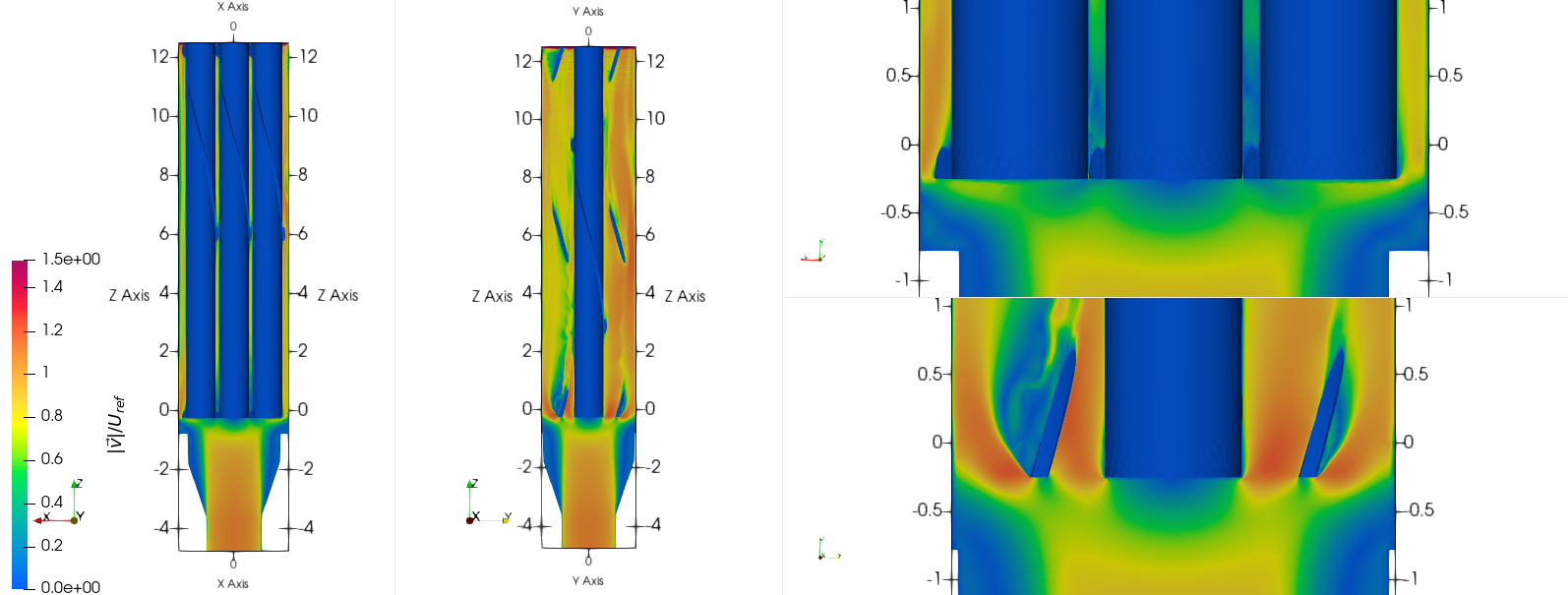
Fig. 26 Normalized velocity magnitude along \(x\) and \(y\) cross-sections. Corresponding zoomed views near overlap region (\(z=0\)) shown.

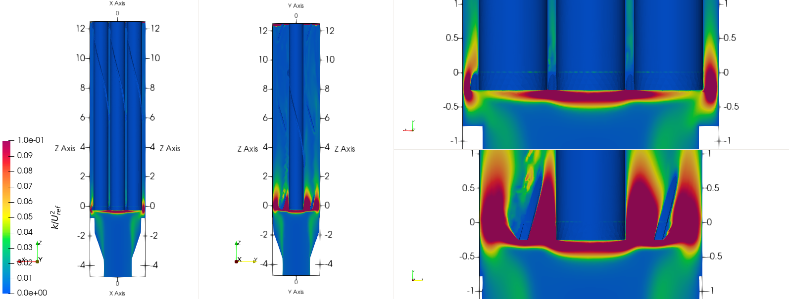
Fig. 27 Normalized TKE along \(x\) and \(y\) cross-sections. Corresponding zoomed views near overlap region (\(z=0\)) shown.

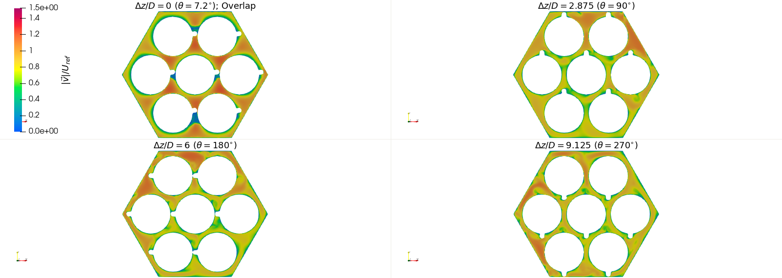
Fig. 28 Normalized velocity magnitude in bundle component at successive downstream locations (corresponding polar orientation annotated).

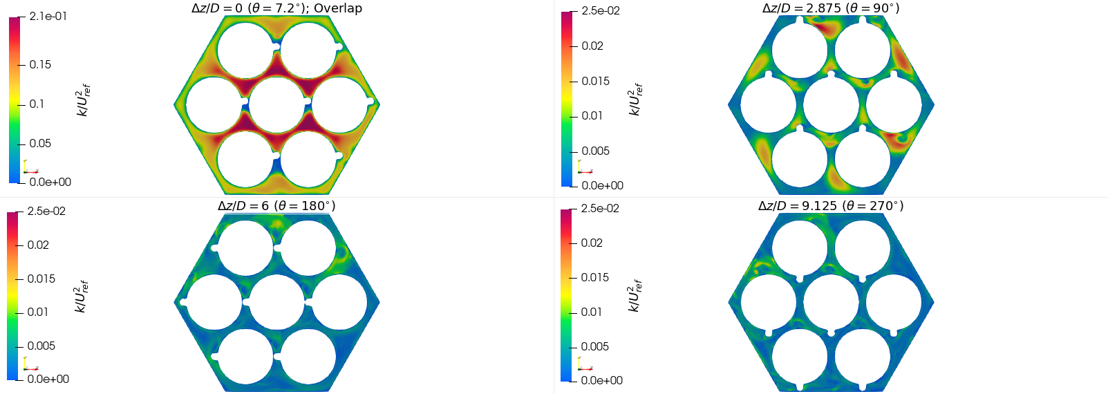
Fig. 29 Normalized TKE in bundle component at successive downstream locations (corresponding polar orientation annotated).

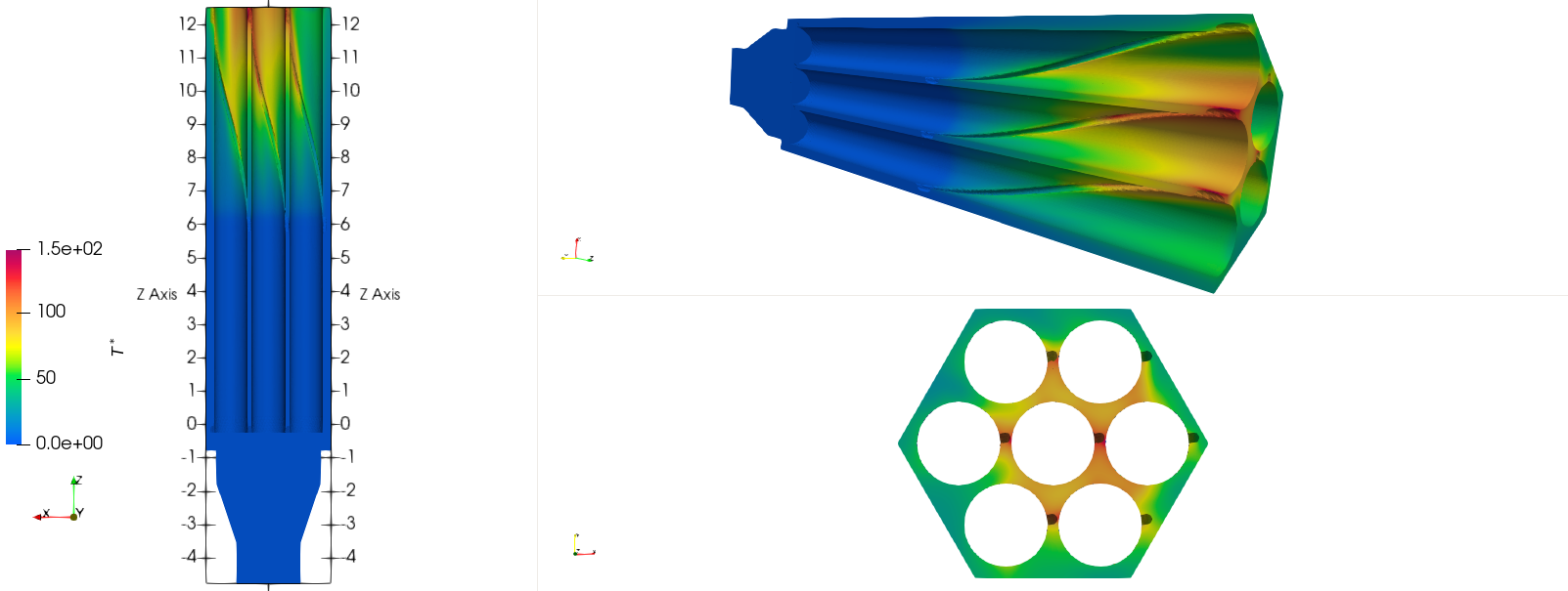
Fig. 30 Dimensionless Temperature contour plot along \(x\) cross-section. Axial cross-section near the outlet also shown.